By Saskia | January 7, 2019
INDperform 
Overview
INDperform is an R package that implements a quantitative framework for selecting and validating the performance of state indicators tailored to meet regional conditions and specific management needs as described in Otto et al. (2018) 1 (see also my post on indicators).
The package builds upon the tidy data principles and offers functions to
- identify temporal indicator changes,
- model relationships to pressures while taking non-linear responses and temporal autocorrelation into account, and to
- quantify the robustness of these models.
These functions can be executed on any number of indicators and pressures. Based on these analyses and a scoring scheme for selected criteria the individual performances can be quantified, visualized, and compared. The combination of tools provided in this package can help making state indicators operational under given management schemes such as the EU Marine Strategy Framework Directive.
Installation
Install the development version from Github using devtools or CRAN:
# install.packages("devtools")
devtools::install_github("saskiaotto/INDperform")
# CRAN:
install.packages("INDperform")
If you encounter a clear bug, please file a minimal reproducible example on github. For questions email me any time.
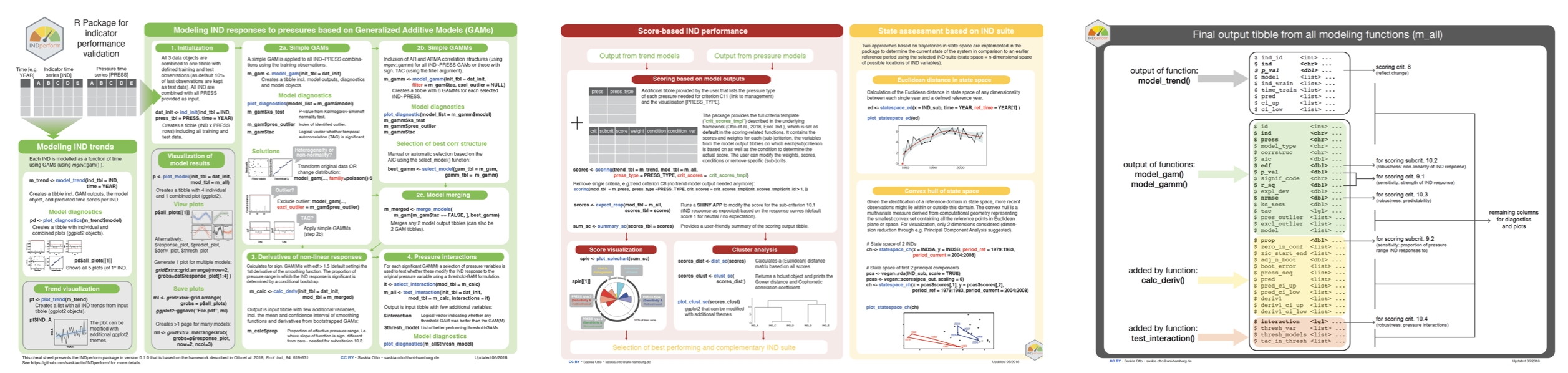
Cheatsheet
Usage
INDperform offers function that can be applied individually to some extent but mostly build upon each other to follow the 7-step process proposed in Otto et al. (2018) (see also the package’s cheat sheet for detailed instructions). For demonstration purposes the package provides a dataset of food web indicators and pressure variables in the Central Baltic Sea (modified from Otto et al., 2018).
This is a suggested workflow demonstrated on the example data included in the package:
library(INDperform)
# Using the demo data
head(ind_ex)
head(press_ex)
head(press_type_ex)
# Scoring template:
crit_scores_tmpl
# Trend modeling -------------
m_trend <- model_trend(ind_tbl = ind_ex[ ,-1],
time = ind_ex$Year)
# Model diagnostics
pd <- plot_diagnostics(model_list = m_trend$model)
pd$all_plots[[1]] # first indicator
# Inspect trends
pt <- plot_trend(m_trend)
pt$TZA # shows trend of TZA indicator
# Indicator response modeling ------------
### Initialize data (combining IND with pressures)
dat_init <- ind_init(ind_tbl = ind_ex[ ,-1],
press_tbl = press_ex[ ,-1], time = ind_ex$Year)
### Model responses
m_gam <- model_gam(init_tbl = dat_init)
# Model diagnostics (e.g. first model)
plot_diagnostics(model_list = m_gam$model[[1]])$all_plots[[1]]
# Any outlier?
m_gam$pres_outlier %>% purrr::compact(.)
# - get number of models with outliers detected
purrr::map_lgl(m_gam$pres_outlier, ~!is.null(.)) %>% sum()
# - which models and what observations?
m_gam %>%
dplyr::select(id, ind, press, pres_outlier) %>%
dplyr::filter(!purrr::map_lgl(m_gam$pres_outlier, .f = is.null)) %>%
tidyr::unnest(pres_outlier)
# Exclude outlier in models
m_gam <- model_gam(init_tbl = dat_init, excl_outlier = m_gam$pres_outlier)
# Any temporal autocorrelation
sum(m_gam$tac)
# - which models
m_gam %>%
dplyr::select(id, ind, press, tac) %>%
dplyr::filter(tac)
# If temporal autocorrelation present
m_gamm <- model_gamm(init_tbl = dat_init,
filter = m_gam$tac)
# Again, any outlier?
purrr::map_lgl(m_gamm$pres_outlier, ~!is.null(.)) %>% sum()
# Select best GAMM from different correlation structures
# (based on AIC)
best_gamm <- select_model(gam_tbl = m_gam,
gamm_tbl = m_gamm)
plot_diagnostics(model_list = best_gamm$model[[1]])$all_plots[[1]]
# Merge GAM and GAMMs
m_merged <- merge_models(m_gam[m_gam$tac == FALSE, ], best_gamm)
# Calculate derivatives
m_calc <- calc_deriv(init_tbl = dat_init,
mod_tbl = m_merged)
# Test for pressure interactions
it <- select_interaction(mod_tbl = m_calc)
# (creates combinations to test for)
m_all <- test_interaction(init_tbl = dat_init, mod_tbl = m_calc,
interactions = it)
# Scoring based on model output ------------
scores <- scoring(trend_tbl = m_trend, mod_tbl = m_all, press_type = press_type_ex)
# Runs a shiny app to modify the score for the subcriterion 10.1:
#scores <- expect_resp(mod_tbl = m_all, scores_tbl = scores)
sum_sc <- summary_sc(scores)
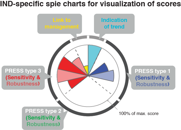
spie <- plot_spiechart(sum_sc)
spie$TZA # shows the spiechart of the indicator TZA
NOTE FOR SPATIAL DATA:
All functions are tailored to indicator time series. Spatial data and spatial autocorrelation testing is currently not included. However, if you have spatial data you could still use all functions except for model_gamm() as it incorporates only temporal autocorrelation structures (AR and ARMA). Simply do the following and use as time vector in ind_init() an integer variable with consecutive numbers (with no gaps!) representing your different stations.
### Use of station numbers instead of time vector
station_id <- 1:nrow(your_indicator_dfr)
dat_init <- ind_init(ind_tbl = your_indicator_dfr,
  press_tbl = your_pressure_dfr, time = station_id)
Validation of IND performances
Modeling IND trends and responses to single pressures
Each IND is modeled as a function of time or a single pressure variable using Generalized Additive Models (GAMs) (based on the mgcv package).
model_trend()models the long-term trend of each IND and returns a tibble with all GAM outputs, the model object, and predicted time series per IND.ind_init()combines the time vector and the IND and press data into one tibble with defined training and test observations. All INDs are combined with all pressures.model_gam()applies GAMs to each IND~pressure combination created inind_init()and returns a tibble including the model output and diagnostics.model_gamm()accounts for temporal autocorrelation in the time series by including correlation structures in the model (using Generalized Additive Mixed Models (GAMMs): AR1, AR2, ARMA1.1, ARMA2.1, ARMA1.2.select_model()selects for each IND~pressure the best correlation structure computed withmodel_gamm()based on the Akaike Information Criterion.merge_models()merges any 2 model output tibbles.calc_deriv()calculates for non-linear responses the 1st derivative of the smoothing function and the proportion of pressure range in which the IND shows a response. Output is input tibble with few additional variables, incl. mean and confidence interval of smoothing function and derivatives from bootstrapped GAMs.test_interaction()tests for each significant GAM(M) whether a selection of pressure variables modifies the IND response to the original pressure using a threshold-GAM formulation. Output is input tibble with few additional variables.
To show the model diagnostics or complete model results
plot_diagnostics()creates a tibble with 6 individual plots (ggplot2 objects) and one combined plot (cowplot object):$cooks_distshows the cooks distance of all observations.$acf_plotshows the autocorrelation function.$pacf_plotshows the partial autocorrelation function.$resid_plotshows residuals vs. fitted values.$qq_plotshows the quantile-quantile plot for normality.$gcvv_plotshows the development of the generalized cross-validation value at different thresholds level of the modifying pressure variable in the threshold-GAM.$all_plotsshows all five (six if threshold-GAM) plots together.
plot_trend()creates a list of ggplot2 objects with all IND trends from the input tibble.plot_model()creates a tibble with 4 individual plots (ggplot2 objects) and one combined plot (cowplot object):$response_plotshows the observed and predicted IND response to the single pressure (based on the training data).$predict_plotshows the test (and train) observations predicted from the model. Included is the normalized root mean square error (NRMSE) for the test data as a measure of model robustness.$deriv_plotshows the first derivative of non-linear IND~pressure response curves and the proportion of the pressure range where the IND shows no further significant change (i.e., slope approximates zero).$thresh_plotshows the IND response curve under a low and high regime of an interacting 2nd pressure variable.$all_plotsshows all plots together.
Scoring IND performance based on model output
Among the 16 common indicator selection criteria, five criteria relate to the indicator’s performances and require time series for their evaluation, i.e.
- Development reflects ecosystem change caused by variation in manageable pressure(s)
- Sensitive or responsive to pressures
- Robust, i.e. responses in a predictive fashion, and statistically sound
- Links to management measures (responsiveness and specificity)
- Relates where appropriate to other indicators but is not redundant
As these are subject to the quality of the underlying data, a thorough determination of whether the indicator as implemented meets the expected requirements is needed. In this package, the scoring scheme for these criteria as proposed by Otto et al. (2018) serves as basis for the quantification of the IND performance. Sensitivity (criterion 9) and robustness (criterion 10) are specified into more detailed sub-criteria to allow for quantification based on statistical models and rated individually for every potential pressure that might affect the IND directly or indirectly.
However, the scoring scheme can easily be adapted to any kind of state indicator and management scheme by modifying the scores, the weighting of scores or by removing (sub)criteria.
crit_scores_tmplThis table contains the scores and weights for each (sub-)criterion. It includes also the variables from the model output tibbles on which each(sub)criterion is based on as well as the condition to determine the actual score. crit_scores_tmpl is set as default in the scoring() function and, if needed, should be modified prior to using the function.
scoring()models the long-term trend of each IND and returns a tibble with all GAM outputs, the model object, and predicted time series per IND.expect_resp()runs a shiny app to modify manually the score for the sub-criterion 10.1 (IND response as expected) based on the response curves (default score 1 for neutral / no expectation).summary_sc()provides a user-friendly summary of the scoring output tibble.plot_spiechart()generates a list of ggplot2 objects (one for each IND). A spie chart superimposes a normal pie chart with a modified polar area chart to permit the comparison of two sets of related data.
Examining redundancies and selecting robust indicator suites
dist_sc()Calculates a (Euclidean) distance matrix based on all scores.clust_sc()applies a hierarchical group-average cluster analysis, returns ahclustobject and prints the Gower distance and Cophonetic correlation coefficient.plot_clust_sc()creates a dendrogram (ggplot2 object) from the cluster analysis.
Assessment of current state status
Two approaches based on trajectories in state space to determine the current state of the system in comparison to an earlier period as reference using the selected IND suite (state space = n-dimensional space of possible locations of IND variables)
Calculation of the Euclidean distance in state space of any dimensionality between each single year (or any other time step used) and a defined reference year.
statespace_ed()calculates the Euclidean distance over time.plot_statespace_ed()creates a ggplot2 object of the Euclidean distance trend.
Given the identification of a reference domain in state space, more recent observations might lie within or outside this domain. The convex hull is a multivariate measure derived from computational geometry representing the smallest convex set containing all the reference points in Euclidean plane or space. For visualization, only 2 dimensions considered (dimension reduction through e.g. Principal Component Analysis suggested).
statespace_ch()calculates the convex hull for 2 defined periods (current and reference) in the x-y space (i.e. 2 IND or 2 Principal Components).plot_statespace_ch()creates a ggplot2 object showing all observed combinations in x-y space as well as the convex hull of both periods. The proportion of the recent time period within the reference space is additionally provided.
Otto, S.A., Kadin, M., Casini, M., Torres, M.A. & Blenckner, T. (2018). A quantitative framework for selecting and validating food web indicators. Ecological Indicators, 84, 619-631, doi: 10.1016/j.ecolind.2017.05.045↩