By Saskia | September 28, 2019

This post compares a few change point detection method available in R given different time series dynamics and research questions. Change points or breakpoints are abrupt variations in time series data and may represent transitions between different states. The detection of change points is useful in modelling and prediction of time series and is found in application areas such as medical condition monitoring, speech and image analysis or climate change detection. In marine ecology, such analysis is often applied to identify sudden shifts in single populations or entire communities and environmental conditions¹. In this case, the change points detection algorithms are applied to single time series and the change points represent simply breaks in time.

More recently, the presence and location of change points (then often termed thresholds) is studied in ecosystem indicators to better interpret and foresee impacts of changes in the intensities of human and environmental pressures². But here, the focus is more on change point in the relationship between a response (i.e. indicator) and explanatory (pressure) variable. But which detection method should be used for this case? I ran into this issue when analyzing indicator-pressure relationships and potential change points for the Baltic Sea. So I started to compare some of the commonly used algorithms by using artificial time series data for which I knew the exact number and location or functional response curve. I thought it might be nice to share the outcome with you and the conclusion I drew from the comparison. I won’t go into too much detail about each package’s function and their settings but I will try to explain a bit more including the R code in the first, real dataset. After that I will only show the numerical and graphical output to be not too lengthy!

Overview

R packages for detecting change points
Summary
Detailed results and R code of detection performance under different scenarios

R packages for detecting change points

The following packages available on CRAN will be compared:

changepoint: changes in mean and variance of time series
bcp: changes in mean; Bayesian approach
strucchange: changes in (time series) regression model
segmented: changes in regression (does not have to be time series data)
tree: classification or regression tree

The changepoint package provides many methods for performing change point analysis of univariate time series³. Although the package only considers the case of independent observations, the theory behind the implemented methods allows for certain types of serial dependence. For specific methods, the expected computational cost can be shown to be linear with respect to the length of the time series. Currently, the changepoint package is only suitable for finding changes in mean or variance. This package also estimates multiple change points through the use of penalization. The drawback to this approach is that it requires a user specified penalty term. A nice tutorial by Rebecca Killick can be found here. The core function I will use here is cpt.mean() with

the default AMOC method for single changepoint detection
the PELT method for detecting multiple changepoints setting the penalty type to AIC and CROPS

The bcp package is designed to perform Bayesian single change point analysis of univariate time series⁴. It returns the posterior probability of a change point occurring at each time index in the series. Recent versions of this package have reduced the computational cost from quadratic to linear with respect to the length of the series. However, all versions of this package are only designed to detect changes in the mean of independent Gaussian observations with its core function bcp().

The strucchange package provides a suite of tools for detecting changes within linear regression models⁵. Many of these tools however, focus on detecting at most one change within the regression model. This package also contains methods that perform online change detection, thus allowing it to be used in settings where there are multiple changes. Additionally, if the number of changes is known a priori then the breakpoint method can be used to perform retrospective analysis. For a given number of changes, this method returns the change point estimates which minimizes the residual sum of squares. There are 3 approaches I will use here:

tests from the generalized fluctuation test (GFT) framework that can detect various types of structural changes: efp() and sctest()
test from the F test framework, which assume that there is one (un- known) breakpoint: Fstats()
test for simultaneous estimation of multiple breakpoints in time series regression models: breakpoints() → here one cane specify in the formula whether one wants to test for a change in the mean (i.e. the intercept) or in the relationship to an explanatory variable.

The segmented package provides functions for segmented or broken-line models, which are regression models where the relationships between the response and one or more explanatory variables are piecewise linear, namely represented by two or more straight lines connected at specific breakpoints⁶. The number of breakpoints of each segmented relationship must be a priori specified.

An alternative approach are so-called decision trees. These tree-based methods for regression and classification involve stratifying or segmenting the predictor space into a number of simple regions. The value at which the regions are split can also be seen as change points in the predictor. While there are numerous tree methods (e.g. boosting, bagging, random forest) and implementations in R I will here use the simple single decision tree approach that is provided by the tree package.

This list of change point detection methods is surely not exclusive but represents fairly well the methods that have been commonly used to analyze ecological regime shifts in marine systems.

Summary

I will start right with the synthesis of my comparison so you can skip the time- and method-specific outcomes. The list of individual results you’ll find below is actually pretty long as I compare 8 methods on 6 different time series (the first is the internal Nile dataset the others are artificial/ simulated datasets). So to spare you all these tedious plots and numeric outputs I summarized here all results into 1 table and a few figures.

I will start right with the synthesis of my comparison so you can skip the tedious and lengthy outcomes of 8 methods that I test on 1 real and 5 artificial data sets. Here is an overview table that shows for each method and dataset the location of each detected change points.

Table 1: Comparison of number and location (loc) of change points (cpts) across time series dynamics and methods. Orange cells indicate good matches with the true dataset.
Time series (loc of true cpts)	AMOC	PELT-AIC	PELT-CROPS	bcp	GFT (F test)	Breakpoints	segmented	tree
1 change in mean (Nile data, #28)	28	(too many)	(too many)	28	28	28	3	28
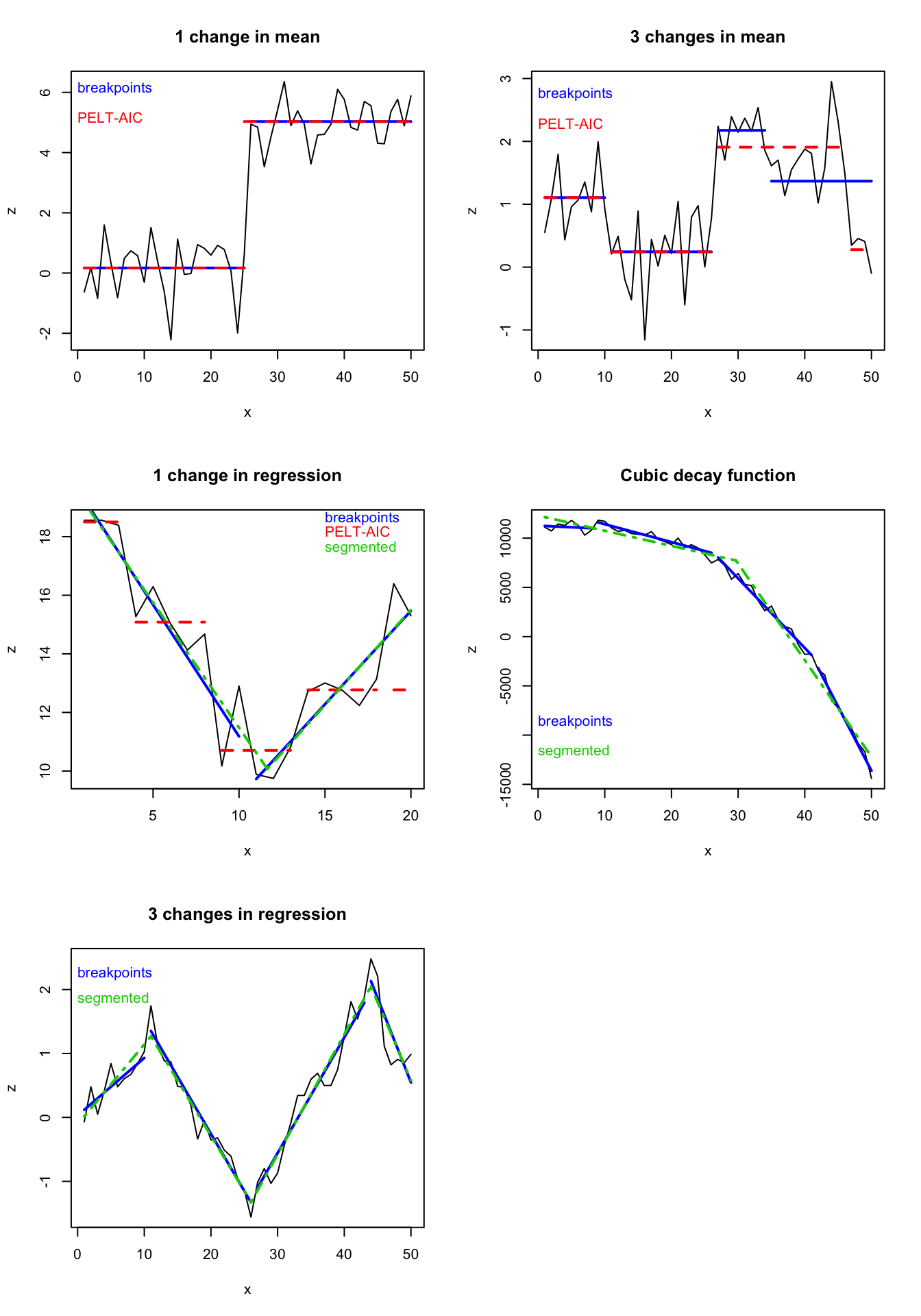
1 change in mean (at #25)	25	25	13,14,23,24,25	25	25	25	14	25
3 changes in mean (at #10,25,45)	none	10,26,46	10,26,46	26	26	10,26,34	20	10,16,26,33,45
1 break in relationship (at #10)	6	3,8,13,18	3,8,13,18	8	8 (6)	10	11	6,14
Cubic decay function	35	(too many)	none	32,43	30 (34)	8,26,41	30	25,35,43
Highly non-linear (4 breaks at #10,25,45)	none	17,32	17,31,39,45	39,45	33 (39)	10,26,43	11,26,44	16,22,32,39,45

Take home message

Obviously there is no one-method-fits-all!
To detect the one major changepoint in the time series several methods can be applied.
But to detect the multiple existing changepoints in dataset 3 only the PELT algorithm (independent of the penalty type) performed well.
The changepoints in the relationship between 2 variables were only detected by the regression breakpoint and segmented algorithm.
Particularly the breakpoints() stands out as it can detect changepoints in means of single time series but also in functional response curves and it does not require any a priori determination of numbers of changepoints!
A good choice might be the complementary use of the PELT algorithm in the changepoint package with the breakpoints method in strucchange.
If one is interested to know when a response variable such as an ecosystem indicator starts to severely deteriorate due to the intensification of a particular human or environmental pressure than regression-based method such as breakpoints or segmented might be a better choice.

For a visual comparison of the better performing models all five artificial time series and the changes in the mean means or relationship are plotted here:

Pros and cons of each method

Changes in mean

changepoint:
- disadvantage here is that one needs to specify a priori if 1 or multiple changes and
- there are many parameters to set which can lead to different results
- when penalty set to “CROPS”, one needs to visually inspect the optimal number of change points
bcp:
- easy to use, not much to specify
- no specification of change points to set a priori
- detection rate depends more on the magnitude of change than other methods
strucchange:
- can cope with many model types, also for changes in means by specifying y ~ 1
- provides confidence intervals of change points
- several test statistics for checking for structural changes: sctest(), Fstats(), breakpoints()
- disav.: sum of the output is tuned to ts object, needs some recoding to adjust to ordinary dataframe (→ applies to sctest(), Fstats())
segmented: useless for changes in mean!
tree:
- the method found all true changepoints
- but unfortunately also some more –> how to choose the optimal one?

Changes in functional curves of relationships between X and Y

strucchange:
- provides several test statistics
- no a priori specification of change points
- provides confidence intervals around the location of the change points!
- allows different type of model structures (but that also requires the correct specification)
segmented:
- disadv.: requires starting values for the change points, hence, one needs to determine the number of change points a priori
- adv.: provides also confidence intervals around the location of the change points!
- disadv.: very simple model structure only allowed

Detailed results and R code of detection performance under different scenarios

# Loading packages
library(changepoint)
library(bcp)
library(strucchange)
library(segmented)
library(tree)

1 change in mean

Real data: Nile dataset

The Nile dataset comes with the R dataset package and represents measurements of the annual flow (in unit 10⁸ m³) of the river Nile at Aswan, between 1871 and 1970. Around 1898, the annual flow dropped greatly from circa 1100 to 800⁷. We will test now whether this shift in 1898 (i.e. in year 28 of the time series) will be detected by all 5 methods.

data(Nile)
str(Nile)

##  Time-Series [1:100] from 1871 to 1970: 1120 1160 963 1210 1160 1160 813 1230 1370 1140 ...

plot(Nile)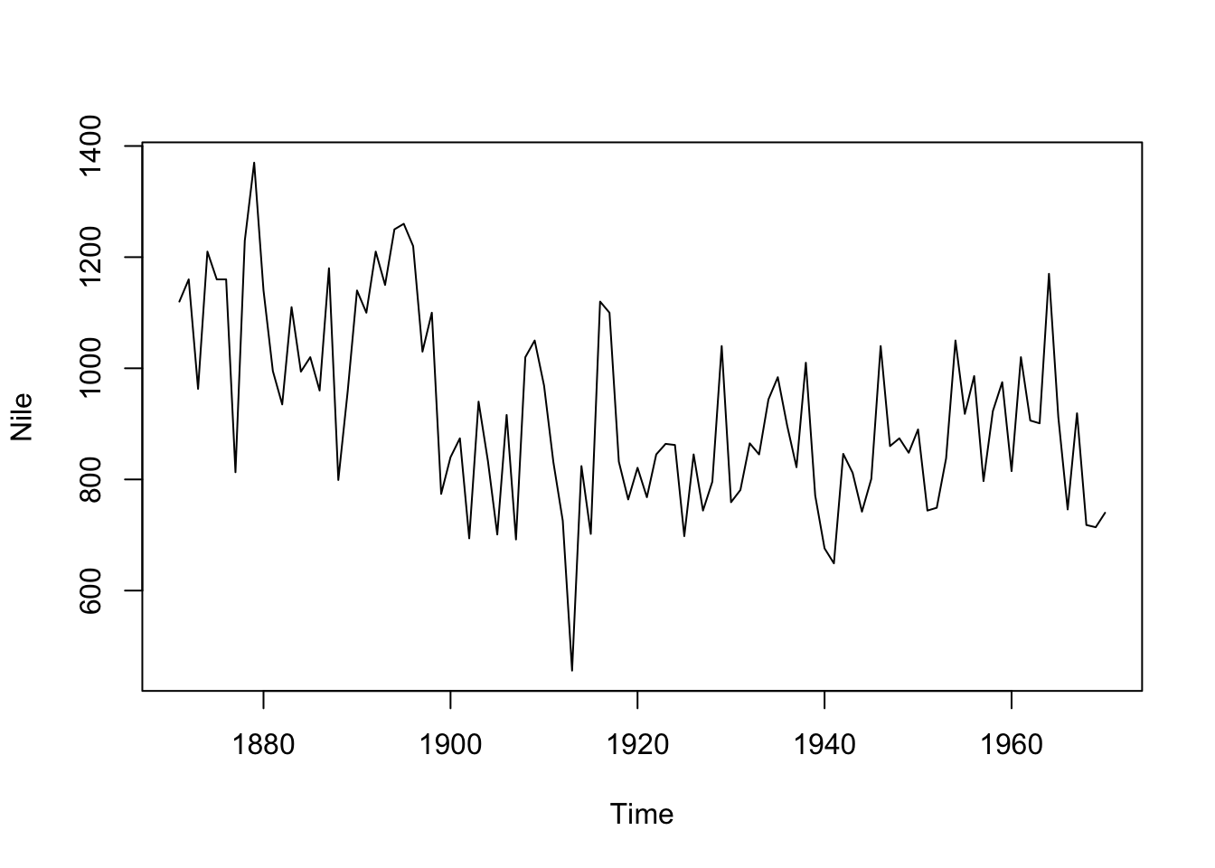

changepoint

Looking for 1 change point using the “AMOC” method (which is also the default):

cpt.mean(Nile, method = "AMOC")

## Class 'cpt' : Changepoint Object
##        ~~   : S4 class containing 12 slots with names
##               cpttype date version data.set method test.stat pen.type pen.value minseglen cpts ncpts.max param.est 
## 
## Created on  : Fri Apr 26 15:58:35 2019 
## 
## summary(.)  :
## ----------
## Created Using changepoint version 2.2.2 
## Changepoint type      : Change in mean 
## Method of analysis    : AMOC 
## Test Statistic  : Normal 
## Type of penalty       : MBIC with value, 13.81551 
## Minimum Segment Length : 1 
## Maximum no. of cpts   : 1 
## Changepoint Locations : 28

The method identifies correctly a change point in 1898 (#28). What would happen when using the setting for identifying multiple change points (if we wouldn’t know the exact number):

cpt.mean(Nile, method = "PELT", Q = 10)

## Class 'cpt' : Changepoint Object
##        ~~   : S4 class containing 12 slots with names
##               cpttype date version data.set method test.stat pen.type pen.value minseglen cpts ncpts.max param.est 
## 
## Created on  : Fri Apr 26 15:58:35 2019 
## 
## summary(.)  :
## ----------
## Created Using changepoint version 2.2.2 
## Changepoint type      : Change in mean 
## Method of analysis    : PELT 
## Test Statistic  : Normal 
## Type of penalty       : MBIC with value, 13.81551 
## Minimum Segment Length : 1 
## Maximum no. of cpts   : Inf 
## Number of changepoints: 94

cpt2 <- cpt.mean(Nile, method = "PELT", penalty = "CROPS", pen.value = c(1,25))

## [1] "Maximum number of runs of algorithm = 6"
## [1] "Completed runs = 2"
## [1] "Completed runs = 3"
## [1] "Completed runs = 5"

summary(cpt2)

## Created Using changepoint version 2.2.2 
## Changepoint type      : Change in mean 
## Method of analysis    : PELT 
## Test Statistic  : Normal 
## Type of penalty       : CROPS with value, 1 25 
## Minimum Segment Length : 1 
## Maximum no. of cpts   : Inf 
## Changepoint Locations :  
## Range of segmentations:
##      [,1] [,2] [,3] [,4] [,5] [,6] [,7] [,8] [,9] [,10] [,11] [,12] [,13]
## [1,]    1    2    3    4    6    7    8    9   10    11    12    13    14
## [2,]    1    2    3    4    6    7    8    9   10    11    12    13    14
## [3,]    1    2    3    4    6    7    8    9   10    11    12    13    14
## [4,]    1    2    3    4    6    7    8    9   10    11    12    13    14
##      [,14] [,15] [,16] [,17] [,18] [,19] [,20] [,21] [,22] [,23] [,24]
## [1,]    15    16    17    18    19    20    21    22    23    24    25
## [2,]    15    16    17    18    19    20    21    22    23    24    25
## [3,]    15    16    17    18    19    20    21    22    23    24    25
## [4,]    15    16    17    18    19    20    21    22    23    24    25
##      [,25] [,26] [,27] [,28] [,29] [,30] [,31] [,32] [,33] [,34] [,35]
## [1,]    26    27    28    29    30    31    32    33    34    35    36
## [2,]    26    27    28    29    30    31    32    33    34    35    36
## [3,]    26    27    28    29    30    31    32    33    34    35    36
## [4,]    26    27    28    29    30    31    32    33    34    35    36
##      [,36] [,37] [,38] [,39] [,40] [,41] [,42] [,43] [,44] [,45] [,46]
## [1,]    37    38    39    40    41    42    43    44    45    46    47
## [2,]    37    38    39    40    41    42    43    44    45    46    47
## [3,]    37    38    39    40    41    42    43    44    45    46    47
## [4,]    37    38    39    40    41    42    43    44    45    46    47
##      [,47] [,48] [,49] [,50] [,51] [,52] [,53] [,54] [,55] [,56] [,57]
## [1,]    48    49    50    51    52    53    54    55    56    57    58
## [2,]    48    49    50    51    52    54    55    56    57    58    59
## [3,]    48    49    50    51    52    54    55    56    57    58    59
## [4,]    48    49    50    51    52    54    55    56    57    58    59
##      [,58] [,59] [,60] [,61] [,62] [,63] [,64] [,65] [,66] [,67] [,68]
## [1,]    59    60    61    62    63    64    65    66    67    68    69
## [2,]    60    61    62    63    64    65    66    67    68    69    70
## [3,]    60    61    62    63    64    65    66    67    68    69    70
## [4,]    60    61    62    63    64    65    66    67    68    69    70
##      [,69] [,70] [,71] [,72] [,73] [,74] [,75] [,76] [,77] [,78] [,79]
## [1,]    70    71    72    73    74    75    76    77    78    79    80
## [2,]    71    72    73    74    75    76    77    78    79    80    81
## [3,]    71    72    73    74    75    76    77    78    79    80    81
## [4,]    71    72    73    74    75    76    77    78    79    80    82
##      [,80] [,81] [,82] [,83] [,84] [,85] [,86] [,87] [,88] [,89] [,90]
## [1,]    81    82    83    84    85    86    87    88    89    90    91
## [2,]    82    83    84    85    86    87    88    89    90    91    92
## [3,]    82    83    84    85    86    87    88    89    90    91    92
## [4,]    83    84    85    86    87    88    89    90    91    93    94
##      [,91] [,92] [,93] [,94] [,95] [,96] [,97] [,98]
## [1,]    92    93    94    95    96    97    98    99
## [2,]    93    94    95    96    97    98    99    NA
## [3,]    93    94    95    96    97    99    NA    NA
## [4,]    95    96    97    99    NA    NA    NA    NA
## 
##  For penalty values: 1 2 8 12.5

We can also plot the diagnostics to see the number of changepoints in each segmentation against the change in test statistic when adding that change. The plot is similar to the scree plot in principal component analysis as when a true changepoint is added the cost increases or decreases rapidly, but when a changepoint due to noise is added the change is small:

plot(cpt2, diagnostic = TRUE)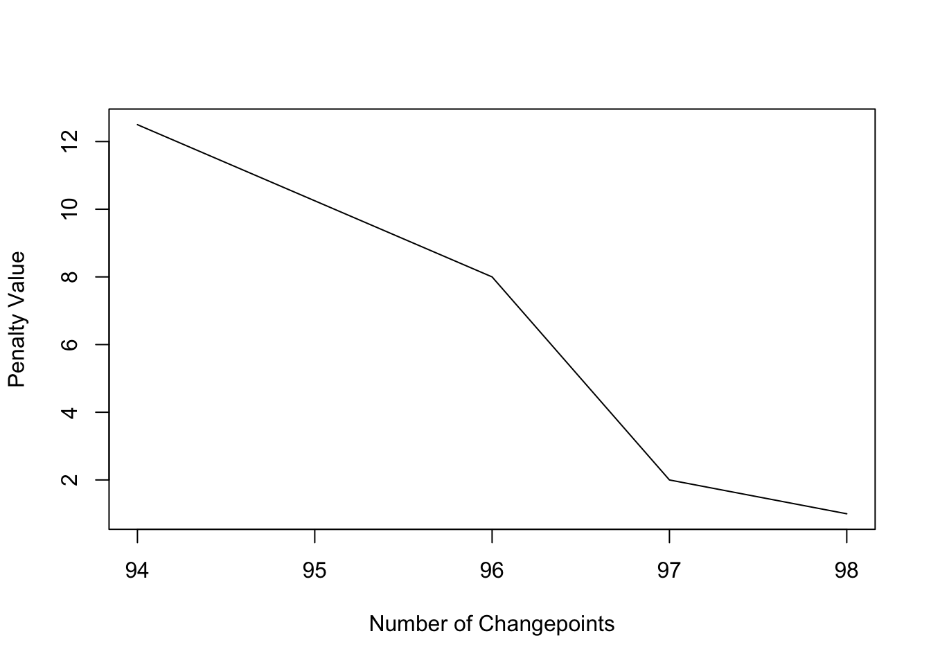

The PELT algorithm detects too many change points (same when methods “SegNeigh” or “BinSeg” were used).

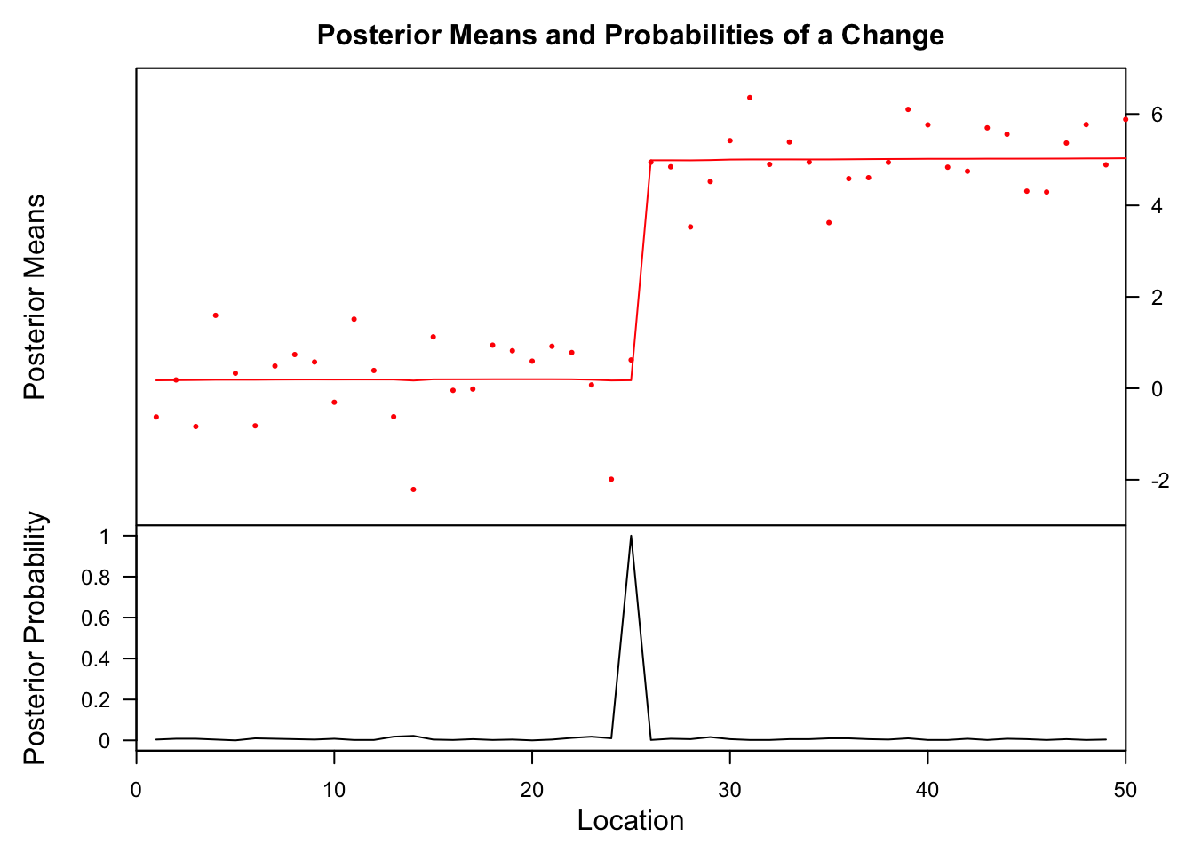
bcp

x <- Nile
bcp_x <- bcp(x, return.mcmc = TRUE)
plot(bcp_x)

The lower posterior probability plot shows that at one location (looks like #28) the probability of a change is very high. We can get the exact locations where probabilities are high (e.g. > 70%) with this code:

bcp_sum <- as.data.frame(summary(bcp_x))
# Let's filter the data frame and identify the year:
bcp_sum$id <- 1:length(x)
(sel <- bcp_sum[which(bcp_x$posterior.prob > 0.7), ])
# Get the year:
time(x)[sel$id]

##    Probability       X1 id
## 28       0.778 1068.629 28

## [1] 1898

Also this method identified the correct year of change.

strucchange

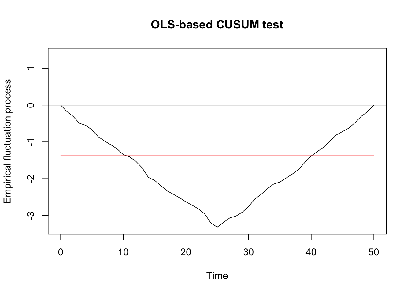
ocus_nile <- efp(Nile ~ 1, type = "OLS-CUSUM")
op <- par(mfrow = c(1,2))
plot(ocus_nile)
plot(ocus_nile, alpha = 0.01, alt.boundary = TRUE)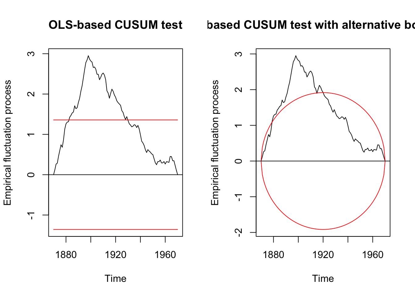

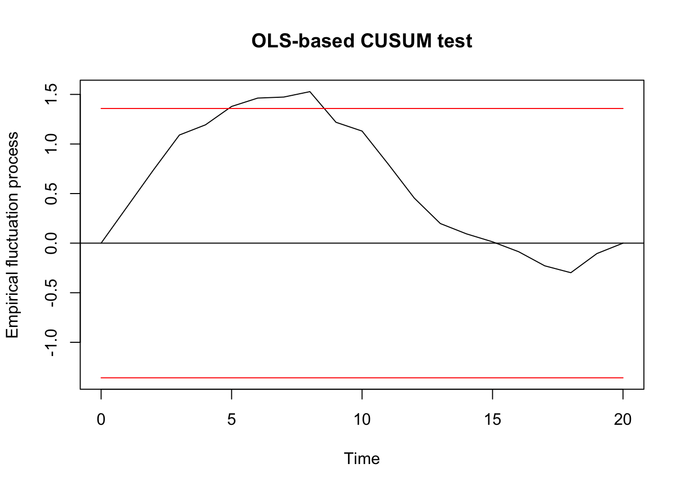
The efp function with the type “OLS-CUSUM” computes an empirical fluctuation process of OLS residuals which is plotted above. The process line shows a peak around 1900 which exceeds the boundaries and, hence, indicates a clear structural shift at that time.

To calculate the corresponding CUSUM and F test statistics for structural change (the first computed on the efp object):

sctest(ocus_nile)

## 
##  OLS-based CUSUM test
## 
## data:  ocus_nile
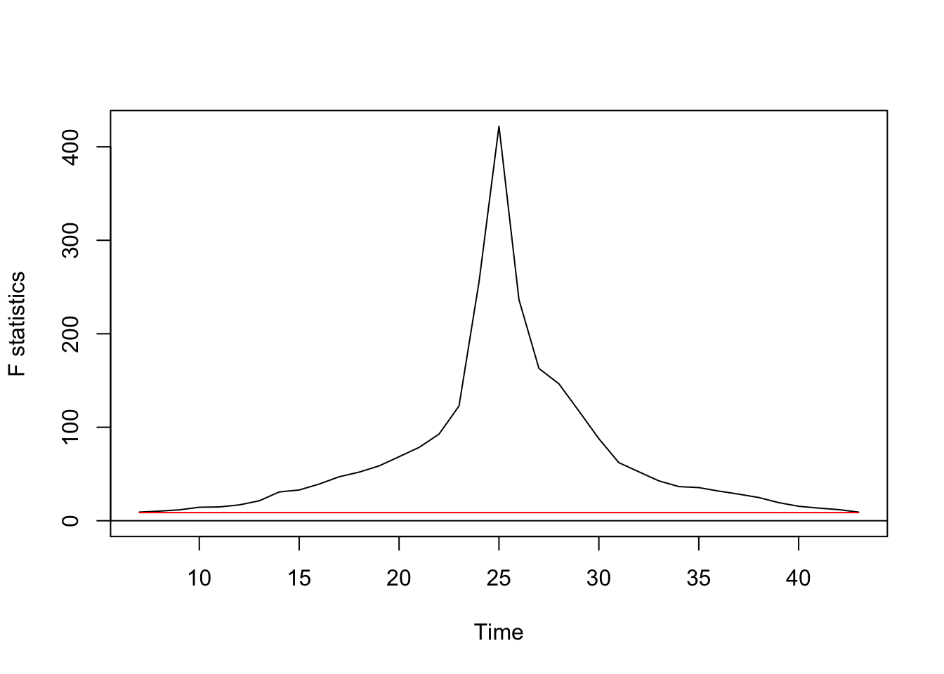
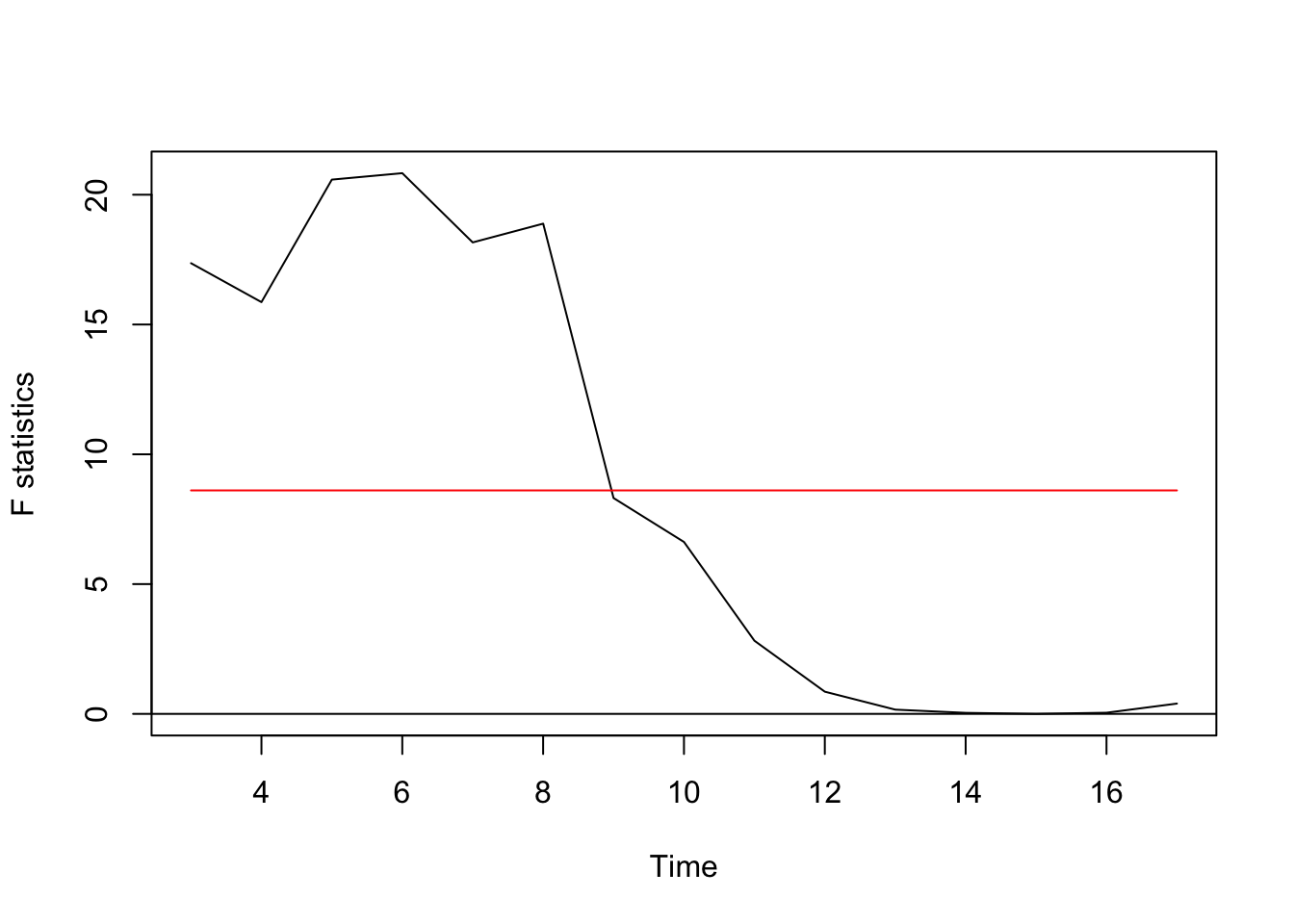
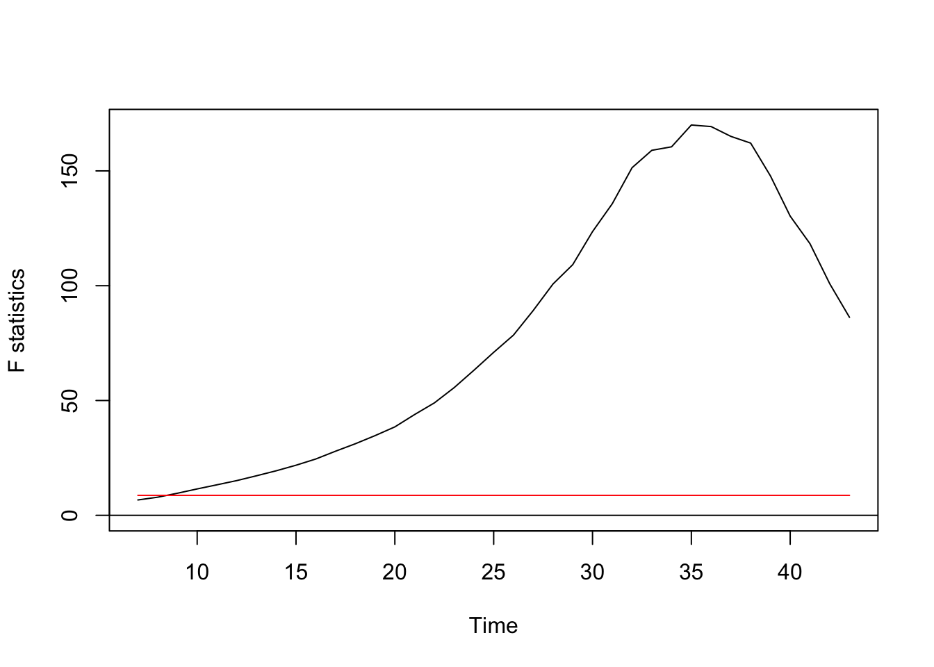
## S0 = 2.9518, p-value = 5.409e-08

fs_nile <- Fstats(Nile ~ 1)
plot(fs_nile)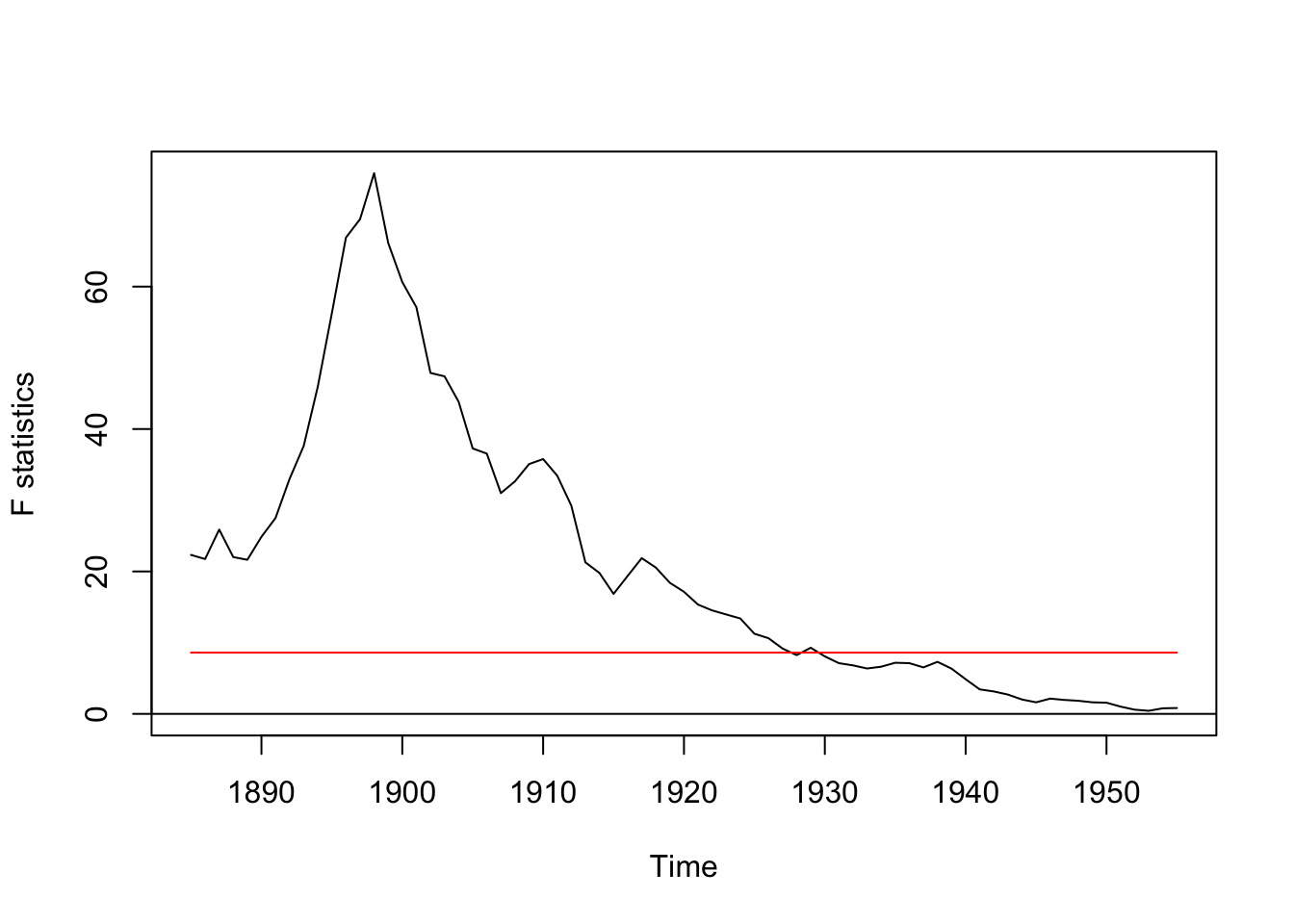

Both tests suggest a significant change in the time series.

Test for 1 breakpoint using the breakpoints() function → Note that the number of breakpoints have to be defined beforehand for this method!

bp_nile <- breakpoints(Nile ~ 1)
bp_nile

## 
##   Optimal 2-segment partition: 
## 
## Call:
## breakpoints.formula(formula = Nile ~ 1)
## 
## Breakpoints at observation number:
## 28 
## 
## Corresponding to breakdates:
## 1898

To check for multiple breaks, the breakpoint() function can be also applied to breakpoints objects with an explicit breaks argument (so you actually nest a breakpoints function in breakpoints():

breakpoints(bp_nile, breaks = 2)

## 
##   Optimal 3-segment partition: 
## 
## Call:
## breakpoints.breakpointsfull(obj = bp_nile, breaks = 2)
## 
## Breakpoints at observation number:
## 28 83 
## 
## Corresponding to breakdates:
## 1898 1953

# Nested syntax with 3 breaks:
breakpoints(breakpoints(Nile ~ 1), breaks = 3)

## 
##   Optimal 4-segment partition: 
## 
## Call:
## breakpoints.breakpointsfull(obj = breakpoints(Nile ~ 1), breaks = 3)
## 
## Breakpoints at observation number:
## 28 68 83 
## 
## Corresponding to breakdates:
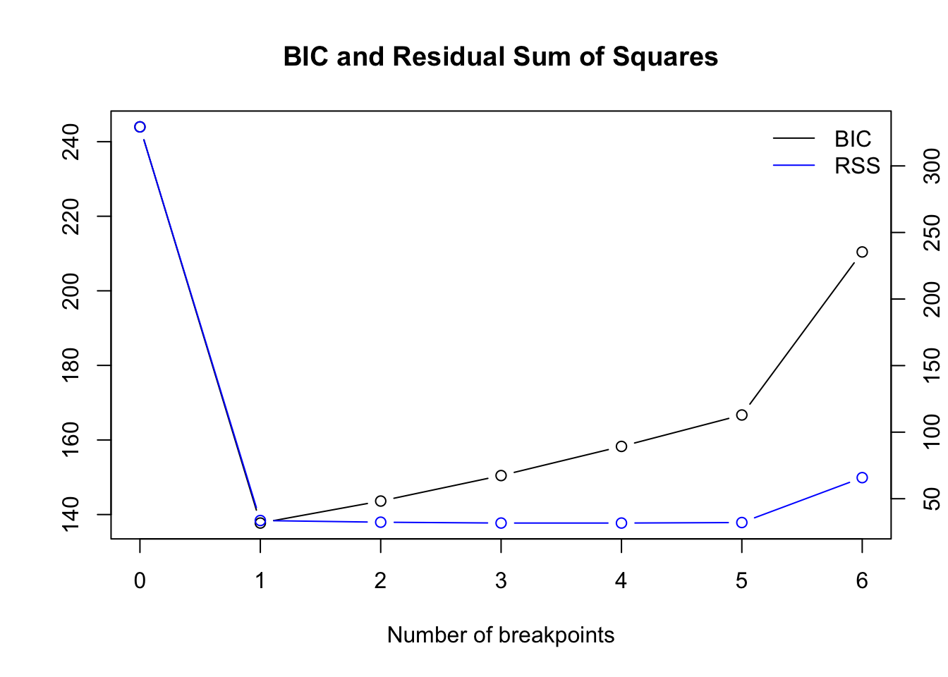
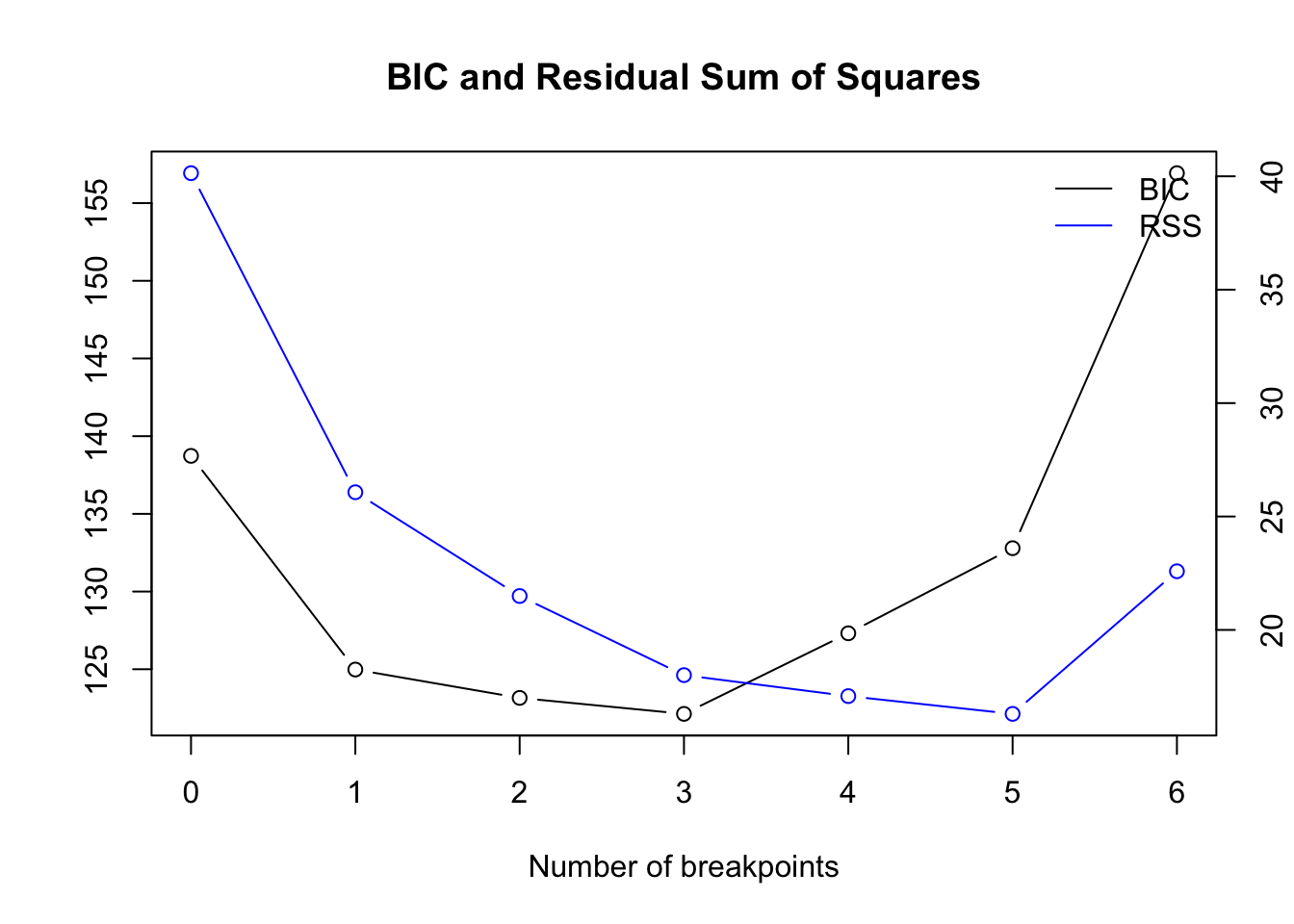
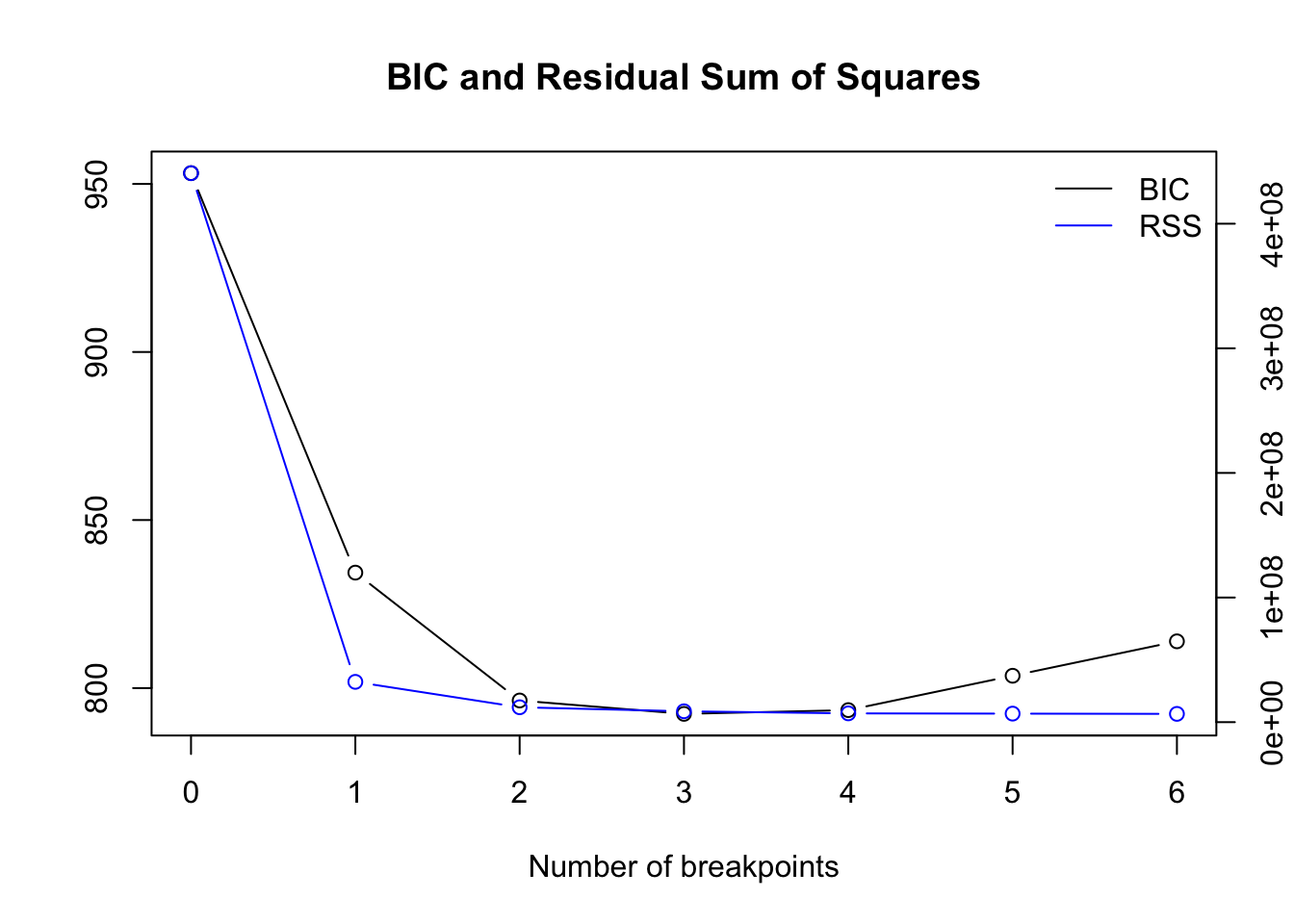
## 1898 1938 1953

So how does one know how many breakpoints exist in the time series? Here, the comparison of BIC estimates for different numbers of breakpoint is useful:

plot(bp_nile)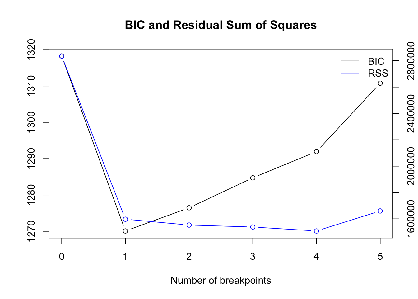

Based on the BIC we should choose one breakpoint.

To get the optimal number numerically instead of inspecting the plot each time, here is a solution:

# get best model
opt_bpts <- function(x) {
  #x = bpts_sum$RSS["BIC",]
  n <- length(x)
  lowest <- vector("logical", length = n-1)
  lowest[1] <- FALSE
  for (i in 2:n) {
    lowest[i] <- x[i] < x[i-1] & x[i] < x[i+1]
  }
  out <- as.integer(names(x)[lowest])
  return(out)
}
bpts_sum <- summary(bp_nile)
opt_brks <- opt_bpts(bpts_sum$RSS["BIC",])
opt_brks

## [1] 1

To get the location of the breakpoint(s):

## [1] 28

One can also visualize the breakpoints in the time series plot with confidence intervals using the stats::confint() function:

ci_nile <- confint(bp_nile, breaks = opt_brks)
plot(Nile)
lines(ci_nile)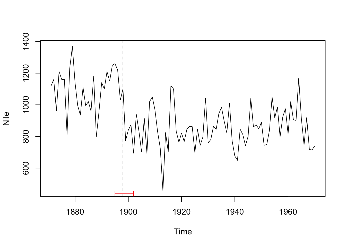

We can also add the regression lines of the null model and our model with 1 breakpoint for comparison:

# null model
fm0 <- lm(Nile ~ 1)
coef(fm0)

## (Intercept) 
##      919.35

# breakpoint model
nile_fac <- breakfactor(bp_nile, breaks = 1)
fm1 <- lm(Nile ~ nile_fac - 1)
coef(fm1)

## nile_facsegment1 nile_facsegment2 
##        1097.7500         849.9722

plot(Nile)
lines(ci_nile)
lines(ts(fitted(fm0), start = 1871), col = 3)
lines(ts(fitted(fm1), start = 1871), col = 4)
lines(bp_nile)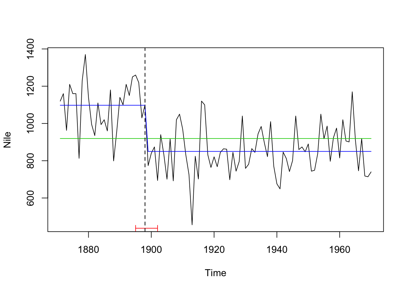

segmented

With this method, the number of breakpoints have to be also specified beforehand similar to the strucchange::breakpoints() function:

Nile_df <- data.frame(Nile = as.numeric(Nile), Year = 1871:1970)
seg_nile <- segmented(lm(Nile ~ 1, data = Nile_df), ~ Year, 
  psi = list(Year = c(1900))) # using 1900 as starting value
summary(seg_nile)

## 
##  ***Regression Model with Segmented Relationship(s)***
## 
## Call: 
## segmented.lm(obj = lm(Nile ~ 1, data = Nile_df), seg.Z = ~Year, 
##     psi = list(Year = c(1900)))
## 
## Estimated Break-Point(s):
##               Est. St.Err
## psi1.Year 1872.98 41.048
## 
## Meaningful coefficients of the linear terms:
##              Estimate Std. Error t value Pr(>|t|)    
## (Intercept) 1147.4404   108.6654  10.559   <2e-16 ***
## U1.Year       -2.7143     0.5404  -5.023       NA    
## ---
## Signif. codes:  0 '***' 0.001 '**' 0.01 '*' 0.05 '.' 0.1 ' ' 1
## 
## Residual standard error: 151.3 on 97 degrees of freedom
## Multiple R-Squared: 0.2165,  Adjusted R-squared: 0.2004 
## 
## Convergence attained in 2 iter. (rel. change 2.0964e-16)

summary(seg_nile)$psi

##           Initial    Est.   St.Err
## psi1.Year    1900 1872.98 41.04761

plot(Nile ~ Year, data = Nile_df, type = "l")
plot(seg_nile, add=T)
lines(seg_nile,col='red')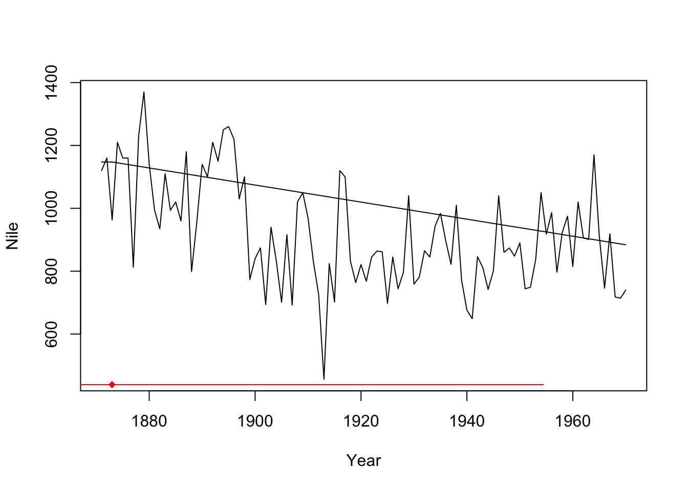

The segmented() function detects one change, but right at the start (1873). It seems to be not devised for this kind of step change.

tree

Nile_df <- data.frame(Nile = as.numeric(Nile), Year = 1871:1970)
tree_nile <- tree(Nile ~ Year, data = Nile_df)
summary(tree_nile)

## 
## Regression tree:
## tree(formula = Nile ~ Year, data = Nile_df)
## Number of terminal nodes:  6 
## Residual mean deviance:  13750 = 1293000 / 94 
## Distribution of residuals:
##     Min.  1st Qu.   Median     Mean  3rd Qu.     Max. 
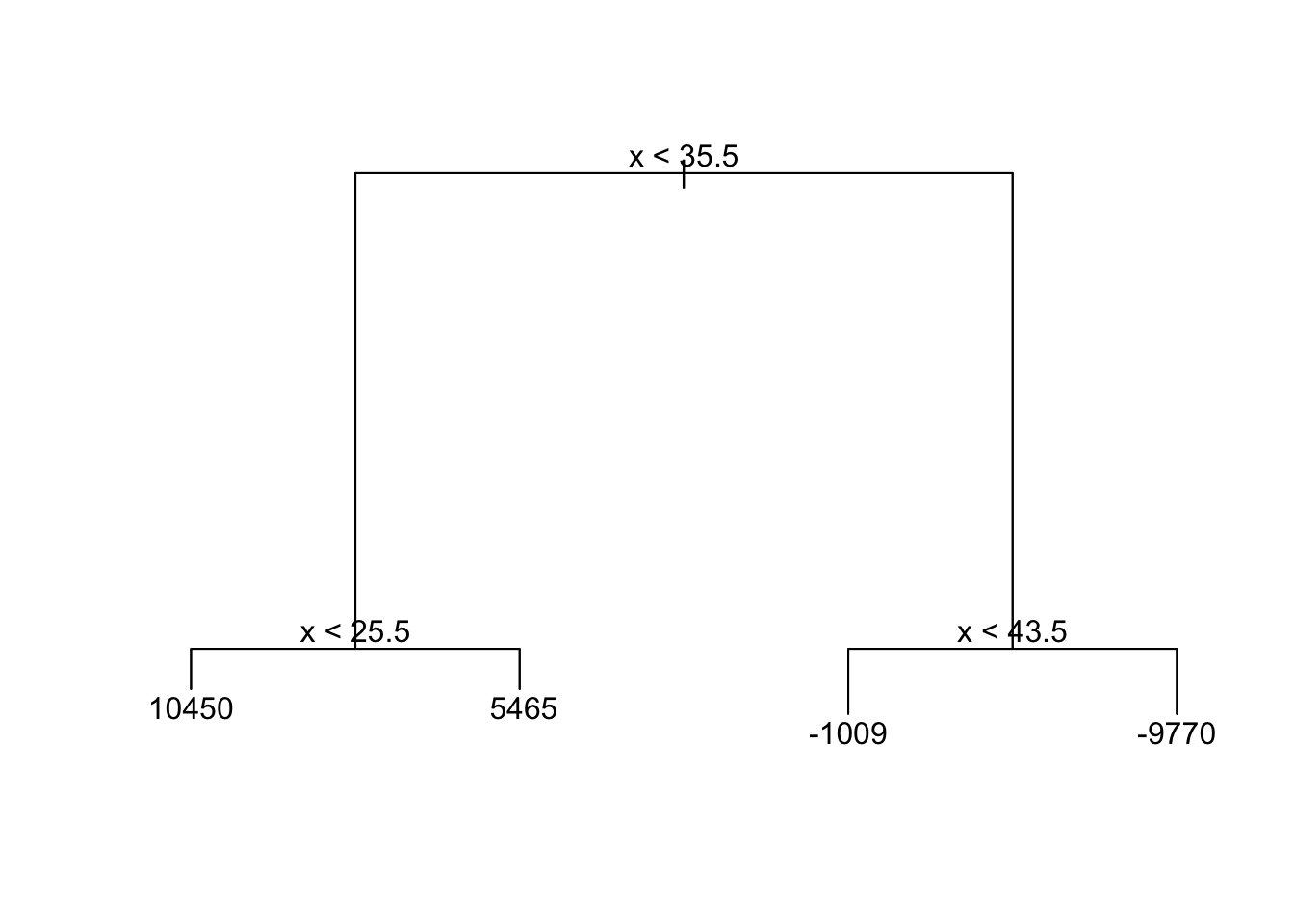
## -380.100  -62.160   -3.645    0.000   54.840  283.900

plot(tree_nile)
text(tree_nile, pretty = 0)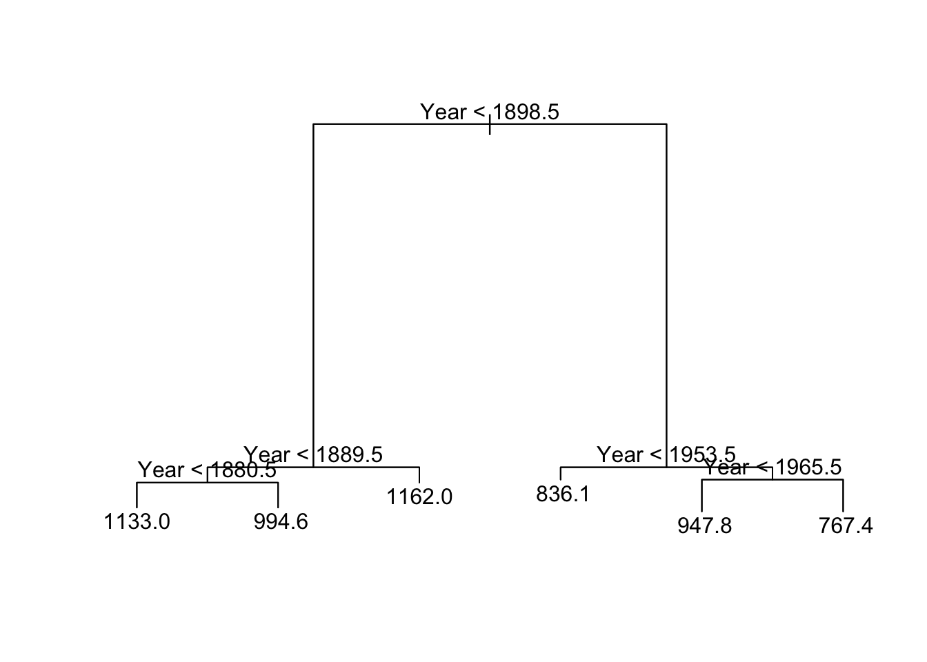

Also the tree() function finds correctly the change point in the Nile time series.

So let’s try another time series…

Artificial data

set.seed(1)
# Normal distributed data with a single change in mean (at x = 25/26)
df <- data.frame(
  x = 1:50,
  z = c(rnorm(25,0,1), rnorm(25,5,1))
)
plot(df$x, df$z, type = 'l', xlab = '', ylab = '')
lines(x = 1:25, y = rep(0,25), col = 'red', lwd = 3)
lines(x=26:50, y = rep(5,25), col = 'red', lwd = 3)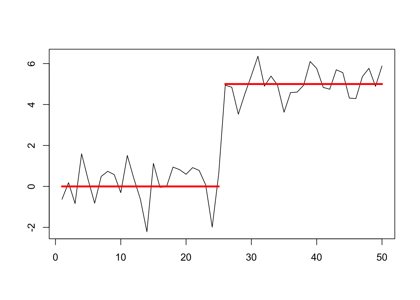

Since it is difficult to identify the location of change points if data input objects for efp() and Fstats() are not a time series, I will convert df$z and use z_ts similar to the Nile data (this will help identifying the row in the data of the changepoint location):

z_ts <- as.ts(df$z)

changepoint

Testing for 1 change point

## Created Using changepoint version 2.2.2 
## Changepoint type      : Change in mean 
## Method of analysis    : AMOC 
## Test Statistic  : Normal 
## Type of penalty       : MBIC with value, 11.73607 
## Minimum Segment Length : 1 
## Maximum no. of cpts   : 1 
## Changepoint Locations : 25

Testing for several using PELT method and AIC penalty:

## Class 'cpt' : Changepoint Object
##        ~~   : S4 class containing 12 slots with names
##               cpttype date version data.set method test.stat pen.type pen.value minseglen cpts ncpts.max param.est 
## 
## Created on  : Fri Apr 26 15:58:35 2019 
## 
## summary(.)  :
## ----------
## Created Using changepoint version 2.2.2 
## Changepoint type      : Change in mean 
## Method of analysis    : PELT 
## Test Statistic  : Normal 
## Type of penalty       : AIC with value, 4 
## Minimum Segment Length : 1 
## Maximum no. of cpts   : Inf 
## Changepoint Locations : 25

Also just 1 change point detected at x = 25.

Testing for several using PELT method and CROPS penalty:

## [1] "Maximum number of runs of algorithm = 13"
## [1] "Completed runs = 2"
## [1] "Completed runs = 3"
## [1] "Completed runs = 5"
## [1] "Completed runs = 9"
## [1] "Completed runs = 11"
## [1] "Completed runs = 12"

## Created Using changepoint version 2.2.2 
## Changepoint type      : Change in mean 
## Method of analysis    : PELT 
## Test Statistic  : Normal 
## Type of penalty       : CROPS with value, 1 25 
## Minimum Segment Length : 1 
## Maximum no. of cpts   : Inf 
## Changepoint Locations :  
## Number of segmentations recorded: 7  with between  1  and  12 changepoints.
##  Penalty value ranges from: 1  to  3.023723

##      [,1] [,2] [,3] [,4] [,5] [,6] [,7] [,8] [,9] [,10] [,11] [,12]
## [1,]    3    4   13   14   23   24   25   29   34    37    44    46
## [2,]    3    4   13   14   23   24   25   29   34    37    NA    NA
## [3,]    3    4   13   14   23   24   25   29   NA    NA    NA    NA
## [4,]    3    4   13   14   23   24   25   NA   NA    NA    NA    NA
## [5,]   13   14   23   24   25   NA   NA   NA   NA    NA    NA    NA
## [6,]   13   14   25   NA   NA   NA   NA   NA   NA    NA    NA    NA
## [7,]   25   NA   NA   NA   NA   NA   NA   NA   NA    NA    NA    NA

CROPS does not give an optimal set of changepoints, thus, we may wish to explore further by looking at the diagnostic plot and the associated penalty transition points:

plot(cpt2, diagnostic = TRUE)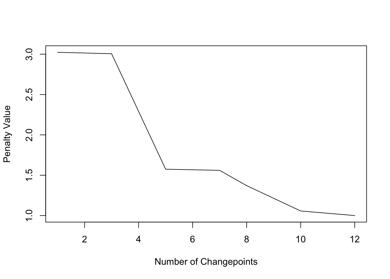

With the PELT method and CROPS penalty 5 change points are detected. So the choice of penalty can be highly relevant.

bcp

##    Probability       X1 id
## 25           1 0.176899 25

strucchange

Generalized fluctuation test

## 
##  OLS-based CUSUM test
## 
## data:  ocus_mod
## S0 = 3.3164, p-value = 5.593e-10

F test

Regression break points

Optimal number of breakpoints:

## [1] 1

Location of breakpoint:

## [1] 25

ci_mod <- confint(bpts, breaks = opt_brks)
plot(z ~ x, data = df, type = "l")
for (i in 1: opt_brks) {
  abline(v = df$x[ci_mod$confint[i,2]], col = "blue")
  abline(v = df$x[ci_mod$confint[i,1]], col = "red", lty = 3)
  abline(v = df$x[ci_mod$confint[i,3]], col = "red", lty = 3)
}

## fit null hypothesis model and model with 1 breakpoint
fm0 <- lm(z ~ 1, data = df)
x_fac <- breakfactor(bpts2, breaks = 1)
fm1 <- lm(z ~ x_fac - 1, data = df)
fm1_coef <- coef(fm1) 

fit1 <- fitted(fm1)[1:best_brk]
fit2 <- fitted(fm1)[(best_brk+1):max(df$x)]

# add to previous plot
lines(df$x, fitted(fm0), col = 3)
lines(df$x[1:best_brk], fit1, col = "orange")
lines(df$x[(best_brk+1):max(df$x)],fit2, col = "orange")

segmented

lin_mod <- lm(z ~ x, data = df)
segm_mod <- segmented(lin_mod, seg.Z = ~x, psi=20)
summary(segm_mod)$psi

##        Initial     Est.   St.Err
## psi1.x      20 13.99996 5.525805

plot(z ~ x, data = df, pch=16)
plot(segm_mod, add=T)
lines(segm_mod,col='red')

The detected change point lies around 14 with a wide confidence interval.

tree

3 changes in mean

set.seed(2)
# Normal distributed data with 3 change in mean (at x = 10/11, 25/26, 45/46)
df <- data.frame(
  x = 1:50,
  z=c(rnorm(10, 1, sd = 0.5), rnorm(15, 0, sd = 0.5),
    rnorm(20, 2, sd = 0.5), rnorm(5, 0.5 , sd = 0.5))
)
plot(df$x, df$z, type = 'l', xlab = '', ylab = '')
lines(x = 1:10, y = rep(1,10), col = 'red', lwd = 3)
lines(x = 11:25, y = rep(0,15), col = 'red', lwd = 3)
lines(x = 26:45, y = rep(2,20), col = 'red', lwd = 3)
lines(x = 46:50, y = rep(0.5,5), col = 'red', lwd = 3)

z_ts <- as.ts(df$z)

changepoint

Testing for 1 change point → nothing detected

## Created Using changepoint version 2.2.2 
## Changepoint type      : Change in mean 
## Method of analysis    : AMOC 
## Test Statistic  : Normal 
## Type of penalty       : MBIC with value, 11.73607 
## Minimum Segment Length : 1 
## Maximum no. of cpts   : 1 
## Changepoint Locations :

Testing for several using PELT method and AIC penalty → 3 change points detected

## Class 'cpt' : Changepoint Object
##        ~~   : S4 class containing 12 slots with names
##               cpttype date version data.set method test.stat pen.type pen.value minseglen cpts ncpts.max param.est 
## 
## Created on  : Fri Apr 26 15:58:35 2019 
## 
## summary(.)  :
## ----------
## Created Using changepoint version 2.2.2 
## Changepoint type      : Change in mean 
## Method of analysis    : PELT 
## Test Statistic  : Normal 
## Type of penalty       : AIC with value, 4 
## Minimum Segment Length : 1 
## Maximum no. of cpts   : Inf 
## Changepoint Locations : 10 26 46

Testing for several using PELT method and CROP type:

## [1] "Maximum number of runs of algorithm = 9"
## [1] "Completed runs = 2"
## [1] "Completed runs = 3"
## [1] "Completed runs = 5"
## [1] "Completed runs = 8"

## Created Using changepoint version 2.2.2 
## Changepoint type      : Change in mean 
## Method of analysis    : PELT 
## Test Statistic  : Normal 
## Type of penalty       : CROPS with value, 1 25 
## Minimum Segment Length : 1 
## Maximum no. of cpts   : Inf 
## Changepoint Locations :  
## Number of segmentations recorded: 7  with between  0  and  7 changepoints.
##  Penalty value ranges from: 1  to  14.06746

In the following order are change points detected:

cpts_ord(cpts.full(cpt2))

## [1] 26 46 10 15 16 33 43

The diagnostic plot shows that the model with only 3 changepoints is the most parsimonious:

plot(cpt2, diagnostic = TRUE)

plot(cpt2, ncpts = 3)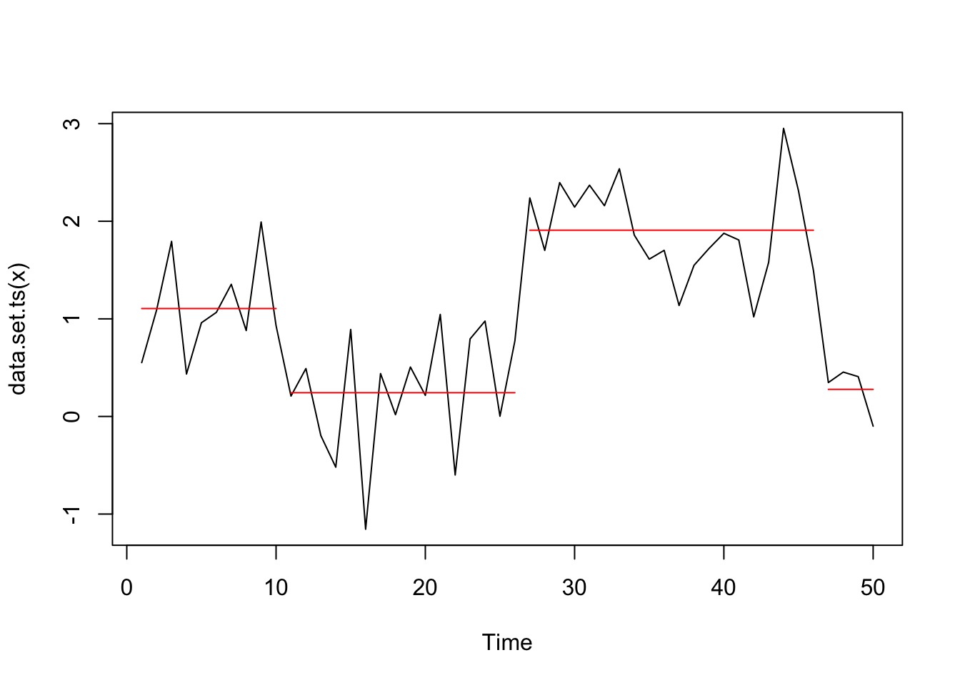

So also with the CROP penalty type we find in this case the 3 changepoints but only when using the diagnostic plot to identify the appropriate number of changes.

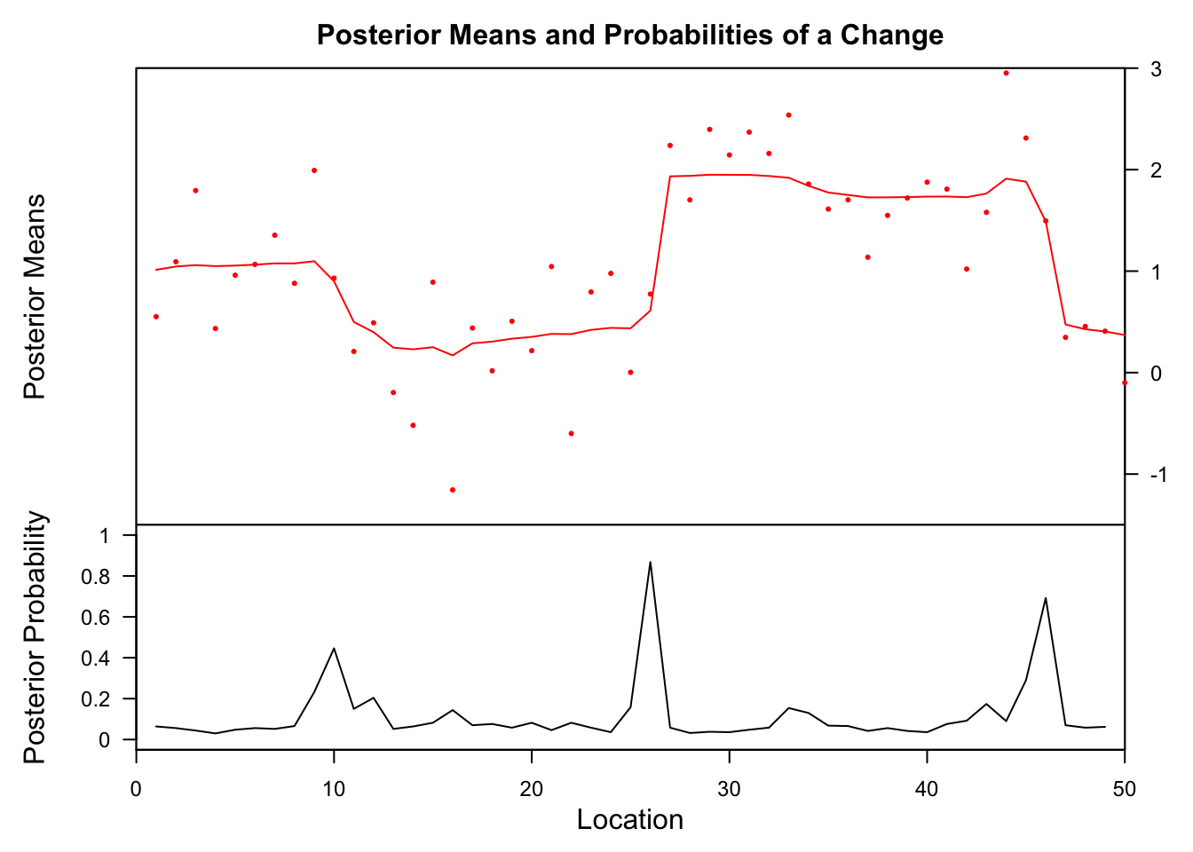
bcp

##    Probability        X1 id
## 26       0.868 0.6111902 26

The highest posterior probabilities for a change are found at location 10, 26 and 46. But only at #26 is the probability higher then 70%, which is considered the minimum to indicate a significant change.

strucchange

Generalized fluctuation test

## 
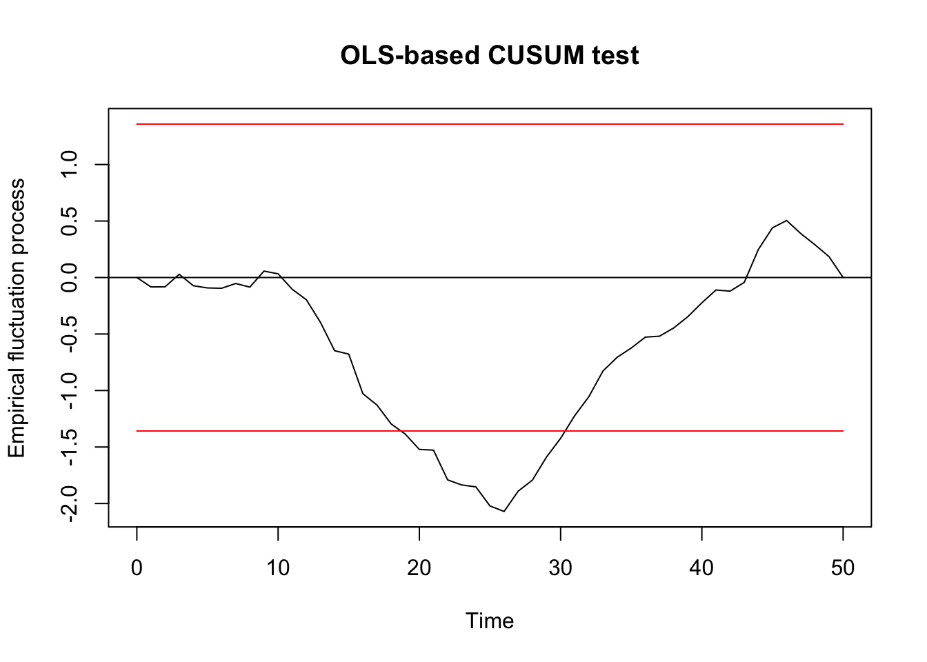
##  OLS-based CUSUM test
## 
## data:  ocus_mod
## S0 = 2.0704, p-value = 0.0003783

F test

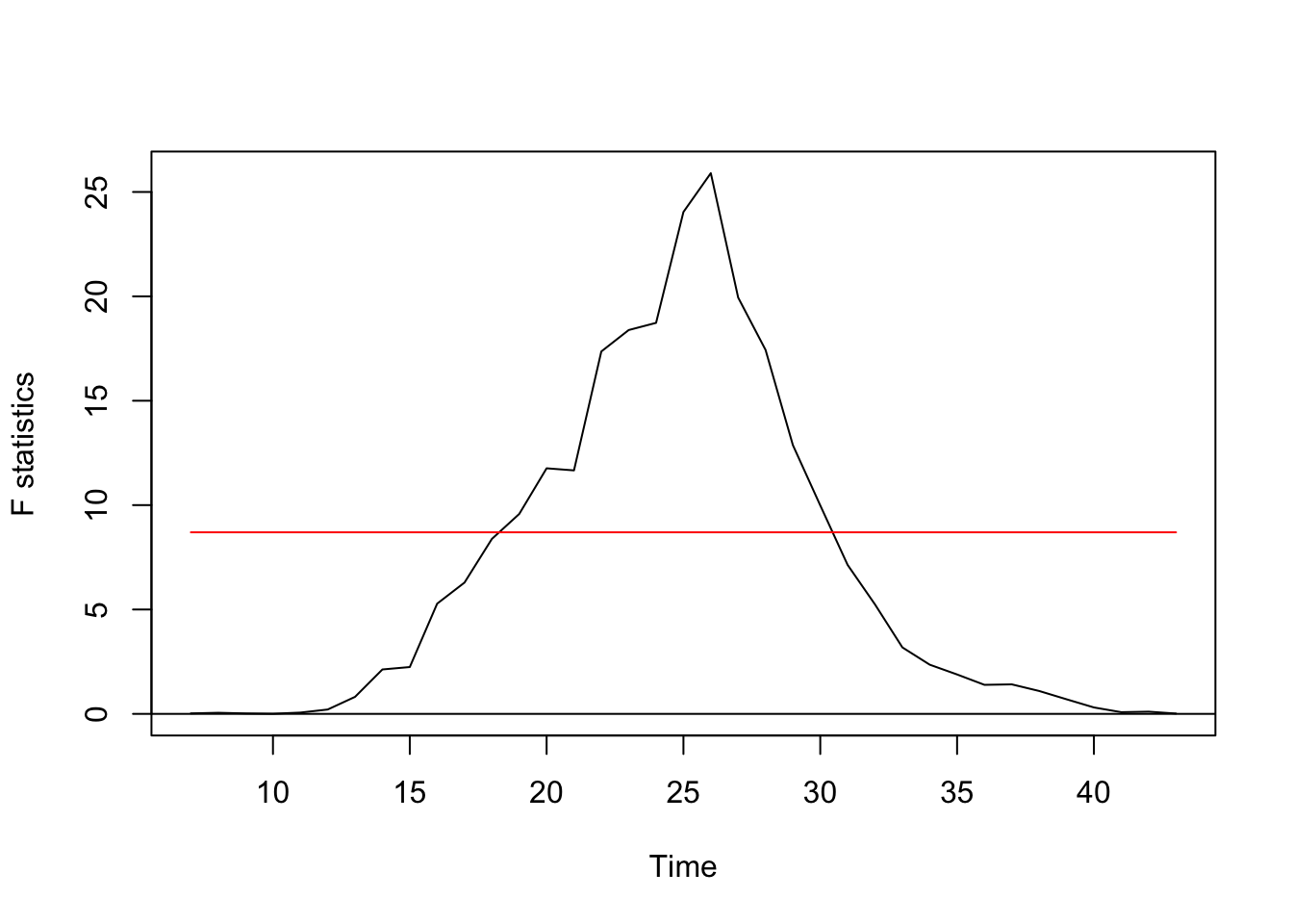
Regression breakpoints

Optimal number of breakpoints:

## [1] 3

Location of breakpoint:

## [1] 10 26 34

While the first 2 frameworks detect only 1 change point, the breakpoints analysis detects all 3 change points but with wider confidence interval:

segmented

##        Initial     Est.  St.Err
## psi1.x      20 44.99772 1.29978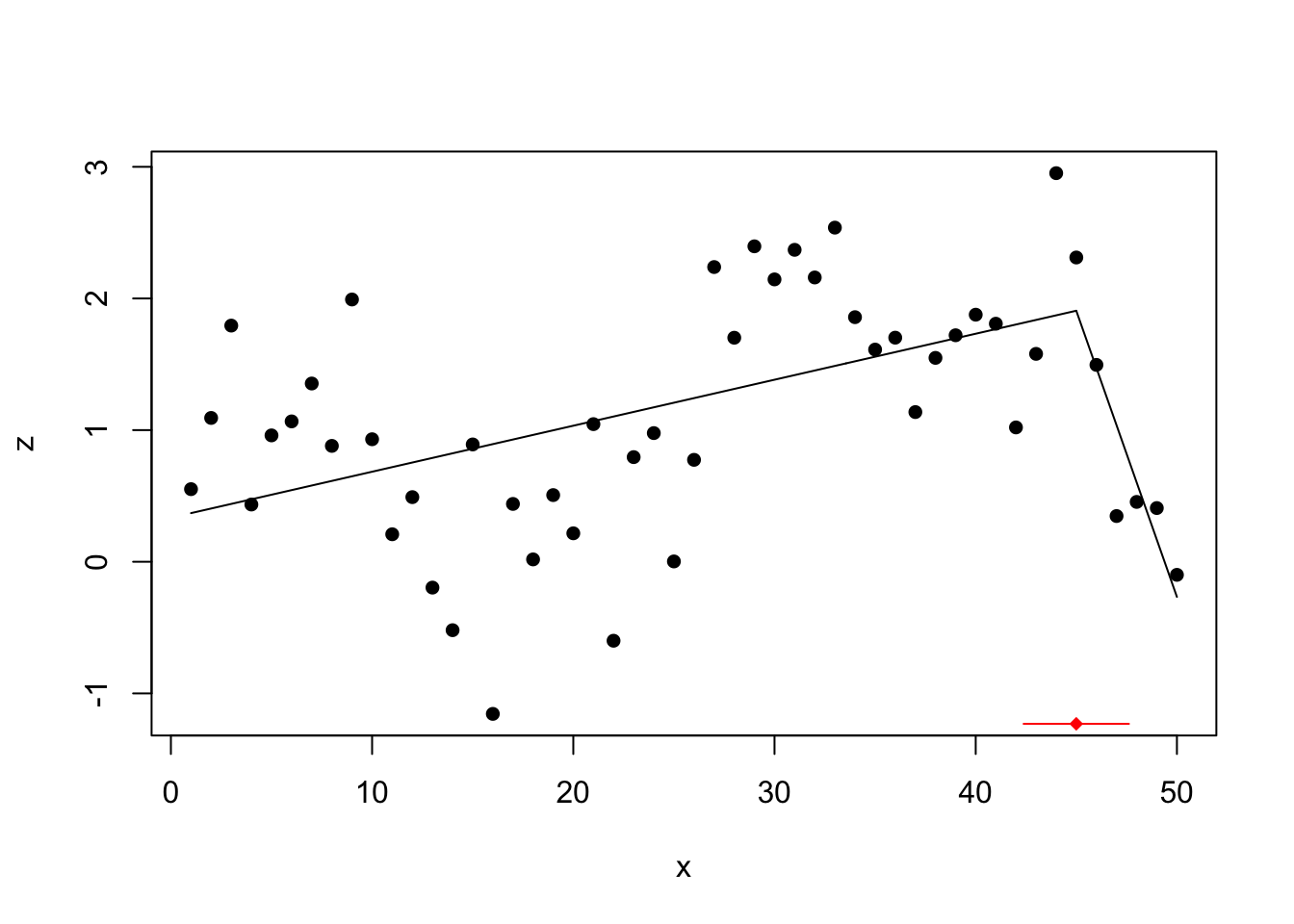

Only the last change point is found with this method.

tree

Linear relationship (z~x) with 1 break

set.seed(3)
z <- numeric(20)
## Create first segment
z[1:10] <- 20:11 + rnorm(10, 0, 1.5)
## Create second segment
z[11:20] <- seq(11, 15, len=10) + rnorm(10, 0, 1.5)
df <- data.frame(x = 1:20, z = z)

plot(df$x, df$z, type='l',xlab='',ylab='')
lines(x = 1:10,y = 20:11, lwd = 3, col = 'red')
lines(x = 11:20, y = seq(11, 15, len=10), lwd = 3, col = 'red')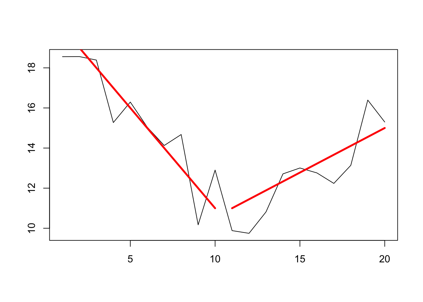

z_ts <- as.ts(df$z)

(changepoints at 10/11)

changepoint

Testing for 1 change point in mean

## Created Using changepoint version 2.2.2 
## Changepoint type      : Change in mean 
## Method of analysis    : AMOC 
## Test Statistic  : Normal 
## Type of penalty       : MBIC with value, 8.987197 
## Minimum Segment Length : 1 
## Maximum no. of cpts   : 1 
## Changepoint Locations : 6

Testing for several using PELT method and AIC penalty:

## Class 'cpt' : Changepoint Object
##        ~~   : S4 class containing 12 slots with names
##               cpttype date version data.set method test.stat pen.type pen.value minseglen cpts ncpts.max param.est 
## 
## Created on  : Fri Apr 26 15:58:35 2019 
## 
## summary(.)  :
## ----------
## Created Using changepoint version 2.2.2 
## Changepoint type      : Change in mean 
## Method of analysis    : PELT 
## Test Statistic  : Normal 
## Type of penalty       : AIC with value, 4 
## Minimum Segment Length : 1 
## Maximum no. of cpts   : Inf 
## Changepoint Locations : 3 8 13 18

Testing for several using PELT method and CROPS penalty:

## [1] "Maximum number of runs of algorithm = 8"
## [1] "Completed runs = 2"
## [1] "Completed runs = 3"
## [1] "Completed runs = 5"
## [1] "Completed runs = 6"
## [1] "Completed runs = 7"

## Created Using changepoint version 2.2.2 
## Changepoint type      : Change in mean 
## Method of analysis    : PELT 
## Test Statistic  : Normal 
## Type of penalty       : CROPS with value, 1 25 
## Minimum Segment Length : 1 
## Maximum no. of cpts   : Inf 
## Changepoint Locations :  
## Number of segmentations recorded: 6  with between  1  and  7 changepoints.
##  Penalty value ranges from: 1  to  24.57129

The diagnostic plot, however, suggest the model with 4 change points as most parsimonious:

plot(cpt2, diagnostic = TRUE)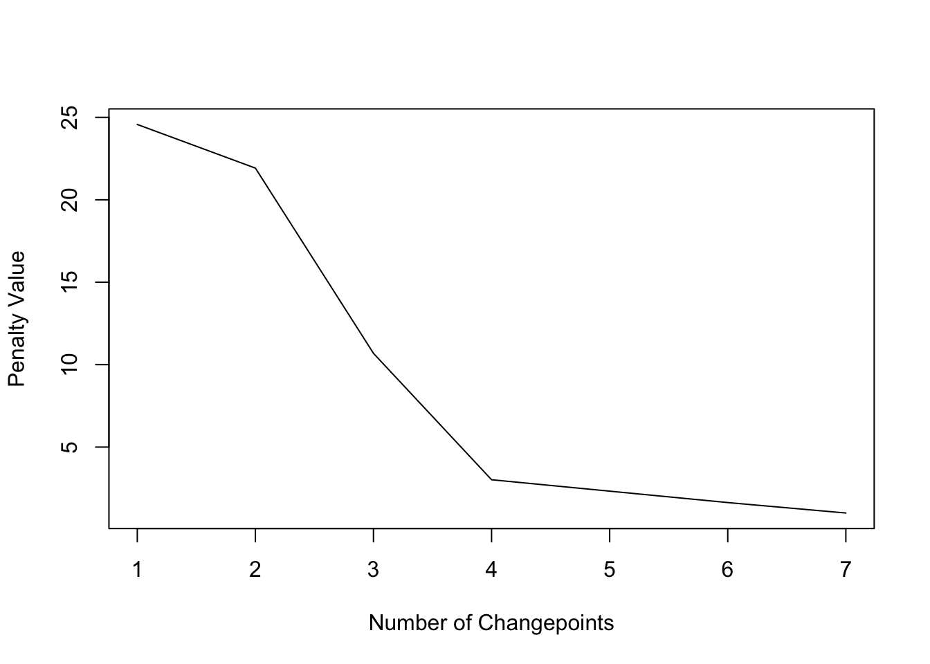

plot(cpt2, ncpts = 4)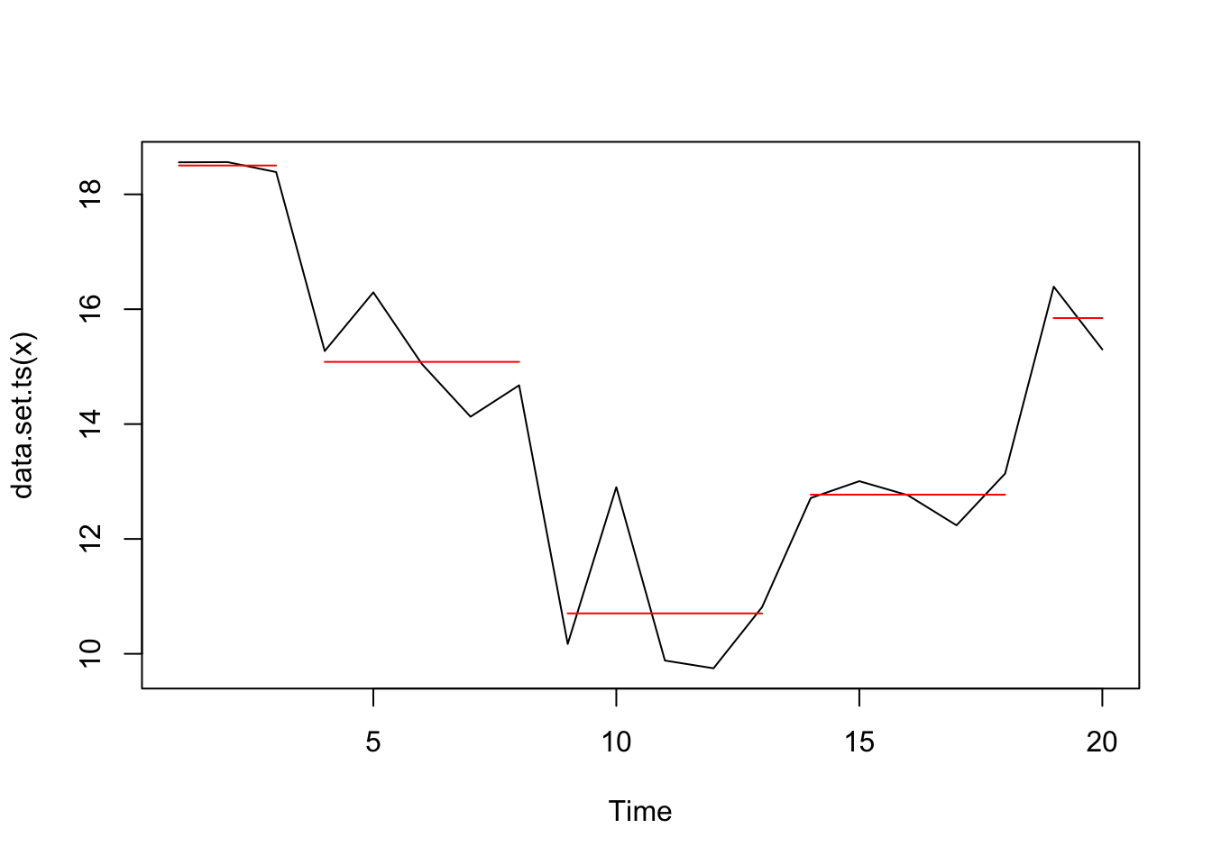

To get the exact locations one has to look at the full matrix of final models found (by row) with their different number of change points:

cpts.full(cpt2)

##      [,1] [,2] [,3] [,4] [,5] [,6] [,7]
## [1,]    3    5    8    9   10   13   18
## [2,]    3    8    9   10   13   18   NA
## [3,]    3    8   13   18   NA   NA   NA
## [4,]    3    8   18   NA   NA   NA   NA
## [5,]    8   18   NA   NA   NA   NA   NA
## [6,]    6   NA   NA   NA   NA   NA   NA

The model with only 4 change points is row 3, so the changepoints are at locations: 3, 8, 13, 18.

bcp

##   Probability       X1 id
## 8       0.746 14.36749  8

The bcp method finds a change point at location 8, which is pretty close to the true value.

strucchange

Generalized fluctuation test

## 
##  OLS-based CUSUM test
## 
## data:  ocus_mod
## S0 = 1.528, p-value = 0.01876

F test

The pattern is less clear here but suggest here optimal change points of 6.

Regression breakpoints

To test for changes in relationships the formula needs to be changed from z~1 to z~x:

bpts <- breakpoints(z ~ x, data = df)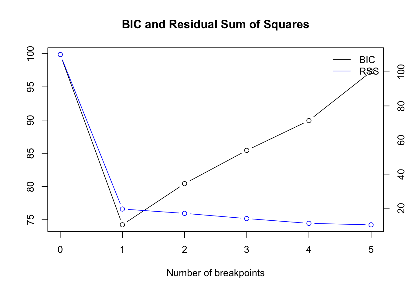

Optimal number of breakpoints:

## [1] 1

Location of breakpoint:

## [1] 10

While the first 2 frameworks detect NO change point, the breakpoints analysis detects it exactly at location 10:

ci_mod <- confint(bpts, breaks = opt_brks)
plot(z ~ x, data = df, type = "l")
for (i in 1: opt_brks) {
  abline(v = df$x[ci_mod$confint[i,2]], col = "blue")
  abline(v = df$x[ci_mod$confint[i,1]], col = "red", lty = 3)
  abline(v = df$x[ci_mod$confint[i,3]], col = "red", lty = 3)
}

## fit null hypothesis model 
fm0 <- lm(z ~ x, data = df)
# fit model with 1 breakpoint but formula different then in previous time series:
fm1 <- lm(z ~ x*(x < best_brk) + x*(x > best_brk), data = df)
fm1_coef <- coef(fm1) 

fit1 <- (fm1_coef[1] + fm1_coef[3]) + (fm1_coef[2] + fm1_coef[5])*df$x[df$x <= best_brk]
fit2 <- (fm1_coef[1] + fm1_coef[4]) + (fm1_coef[2])*df$x[df$x >= best_brk]

# add to previous plot
lines(df$x, fitted(fm0), col = 3)
lines(df$x[1:best_brk], fit1, col = "orange")
lines(df$x[best_brk:max(df$x)], fit2, col = "orange")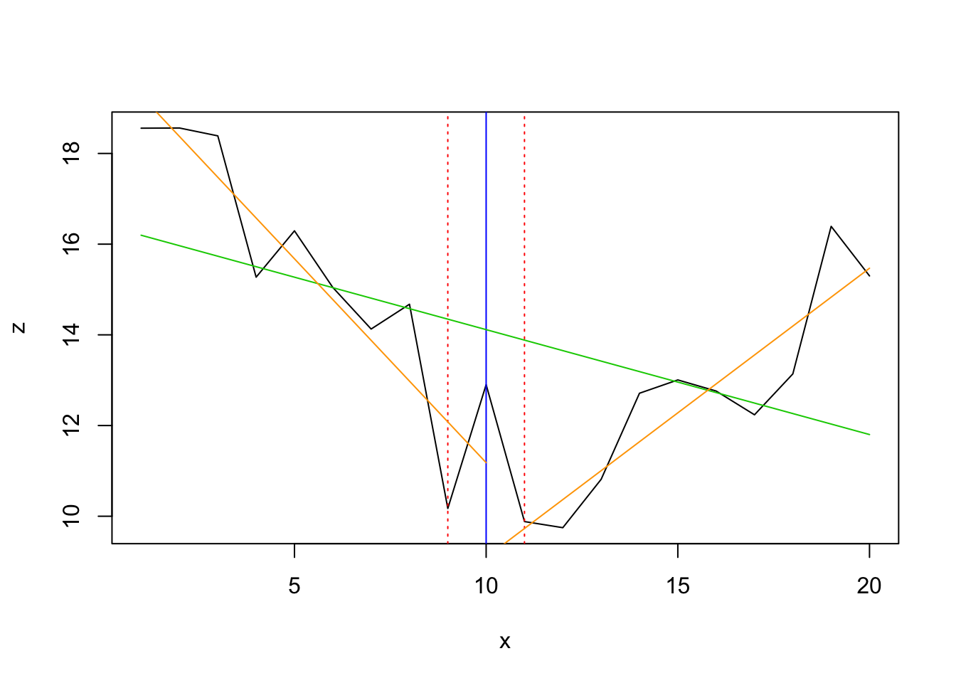

segmented

##        Initial     Est.    St.Err
## psi1.x      10 11.64798 0.6721446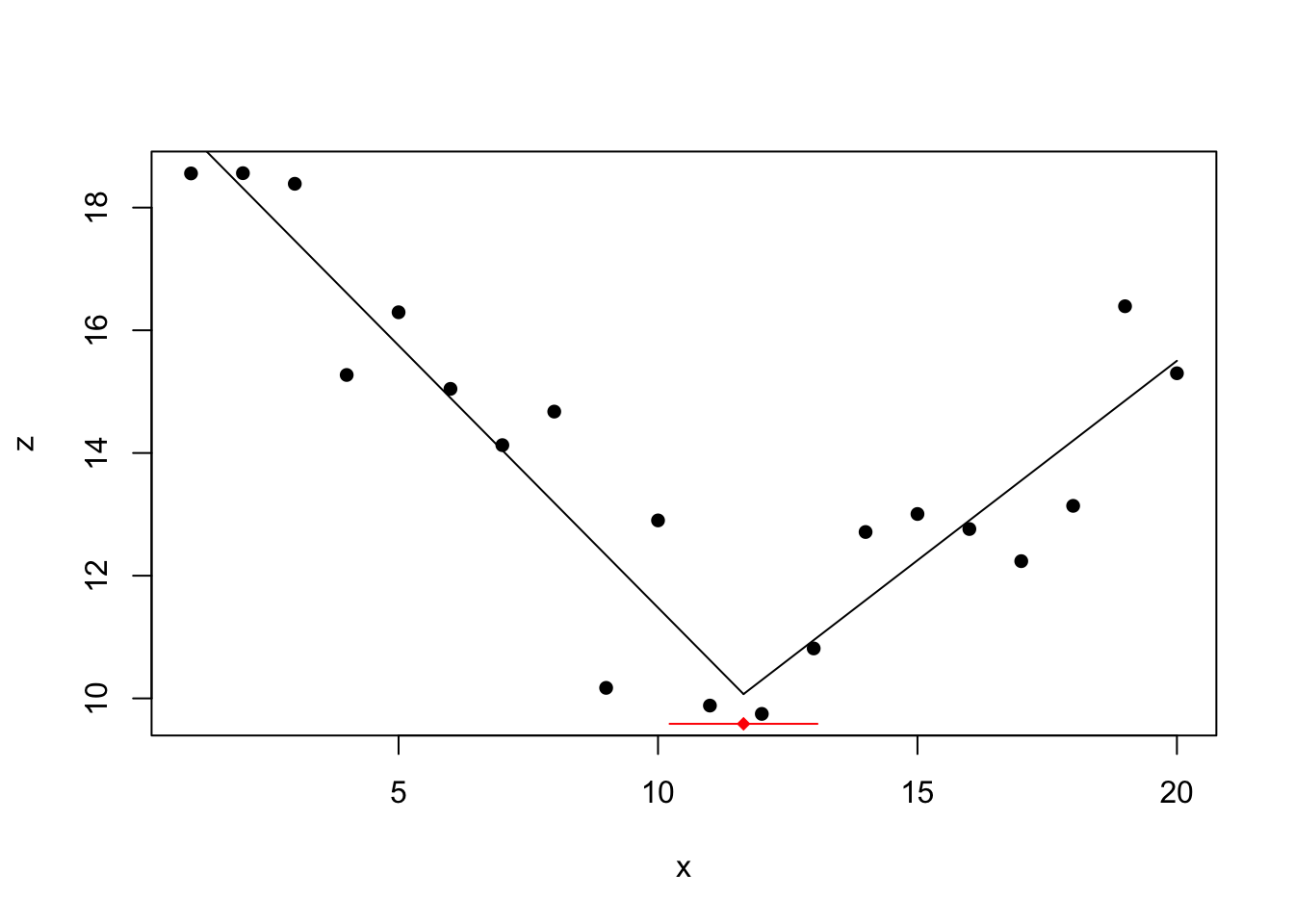

Also the segmented function detects correctly the change at location 10.

tree

This tree methods detects 2 changes which are below and above the true change point.

Cubic decay function (z~x)

set.seed(4)
x <- 1:50
z_nonoise <- (10000 + 0.05*x + 0.2*x^2 - 0.2*x^3)
z <- z_nonoise + rnorm(50,1000,500)
df <- data.frame(x = x, z = z)

plot(df$x, df$z, type = 'l', xlab = '', ylab = '')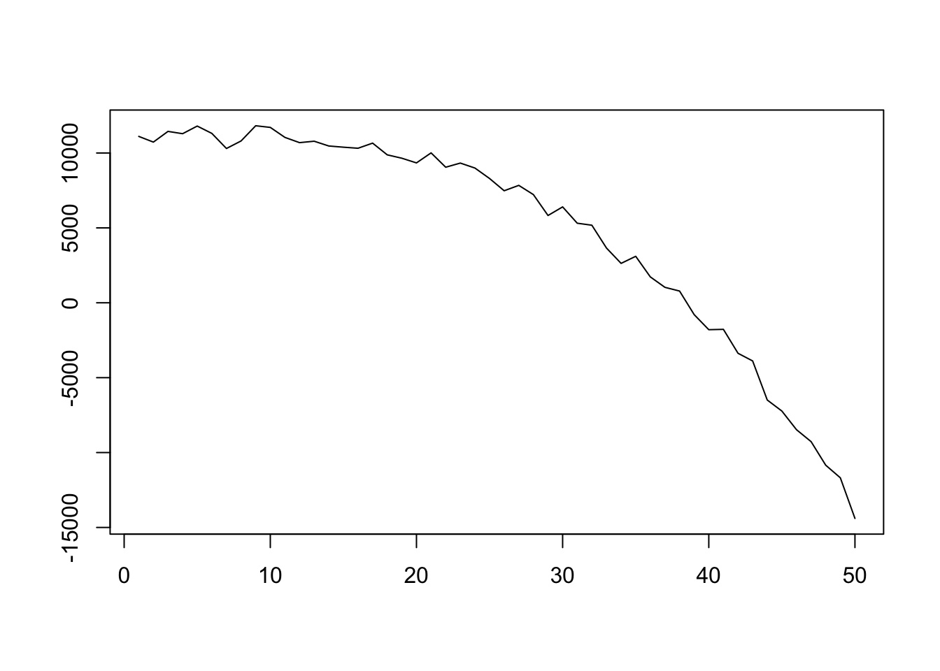

z_ts <- as.ts(df$z)

changepoint

Testing for 1 change point in mean

## Created Using changepoint version 2.2.2 
## Changepoint type      : Change in mean 
## Method of analysis    : AMOC 
## Test Statistic  : Normal 
## Type of penalty       : MBIC with value, 11.73607 
## Minimum Segment Length : 1 
## Maximum no. of cpts   : 1 
## Changepoint Locations : 35

Testing for several using PELT method and AIC penalty:

## Class 'cpt' : Changepoint Object
##        ~~   : S4 class containing 12 slots with names
##               cpttype date version data.set method test.stat pen.type pen.value minseglen cpts ncpts.max param.est 
## 
## Created on  : Fri Apr 26 15:58:35 2019 
## 
## summary(.)  :
## ----------
## Created Using changepoint version 2.2.2 
## Changepoint type      : Change in mean 
## Method of analysis    : PELT 
## Test Statistic  : Normal 
## Type of penalty       : AIC with value, 4 
## Minimum Segment Length : 1 
## Maximum no. of cpts   : Inf 
## Number of changepoints: 49

Testing for several using PELT method and CROPS penalty:

## [1] "Maximum number of runs of algorithm = 2"
## [1] "Completed runs = 2"

## Created Using changepoint version 2.2.2 
## Changepoint type      : Change in mean 
## Method of analysis    : PELT 
## Test Statistic  : Normal 
## Type of penalty       : CROPS with value, 1 25 
## Minimum Segment Length : 1 
## Maximum no. of cpts   : Inf 
## Changepoint Locations :  
## Range of segmentations:
##      [,1] [,2] [,3] [,4] [,5] [,6] [,7] [,8] [,9] [,10] [,11] [,12] [,13]
## [1,]    1    2    3    4    5    6    7    8    9    10    11    12    13
##      [,14] [,15] [,16] [,17] [,18] [,19] [,20] [,21] [,22] [,23] [,24]
## [1,]    14    15    16    17    18    19    20    21    22    23    24
##      [,25] [,26] [,27] [,28] [,29] [,30] [,31] [,32] [,33] [,34] [,35]
## [1,]    25    26    27    28    29    30    31    32    33    34    35
##      [,36] [,37] [,38] [,39] [,40] [,41] [,42] [,43] [,44] [,45] [,46]
## [1,]    36    37    38    39    40    41    42    43    44    45    46
##      [,47] [,48] [,49]
## [1,]    47    48    49
## 
##  For penalty values: 1

Nothing detected.

bcp

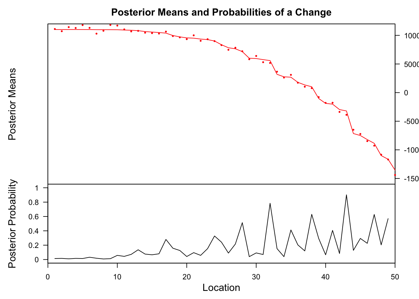
##    Probability        X1 id
## 32       0.784  5591.184 32
## 43       0.902 -3204.395 43

strucchange

Generalized fluctuation test

## 
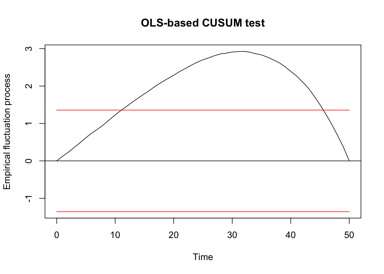
##  OLS-based CUSUM test
## 
## data:  ocus_mod
## S0 = 2.9277, p-value = 7.175e-08

F test

Regression breakpoints

Optimal number of breakpoints:

## [1] 3

Location of breakpoint:

## [1]  8 26 41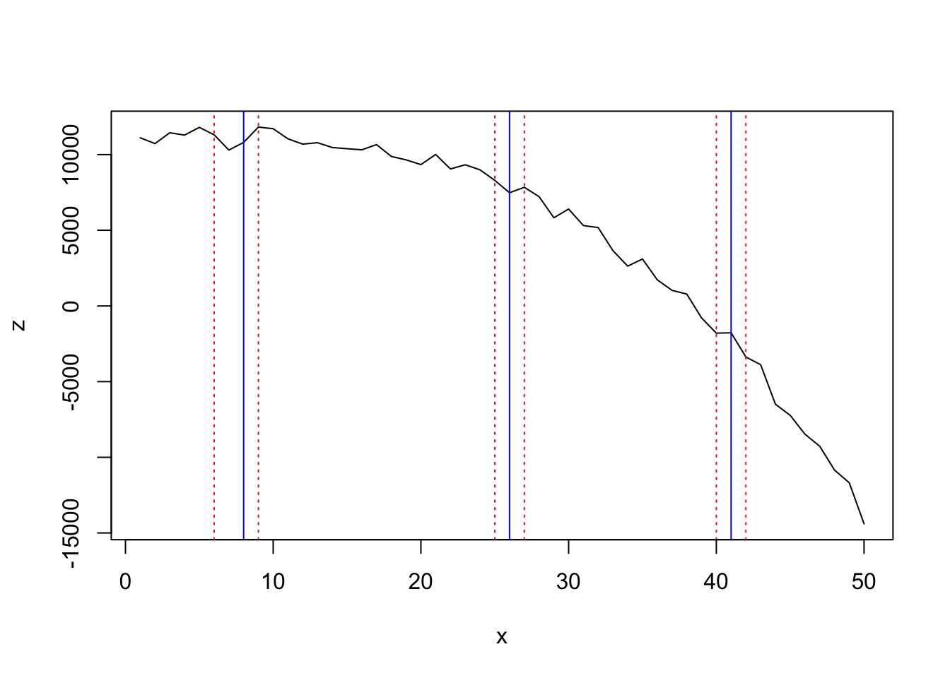

segmented

##        Initial     Est.   St.Err
## psi1.x      10 29.67403 0.579635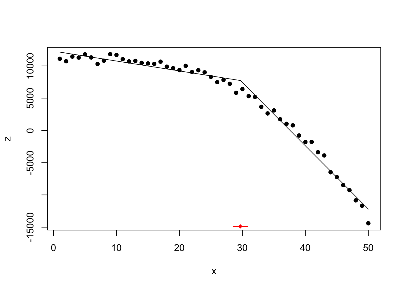

tree

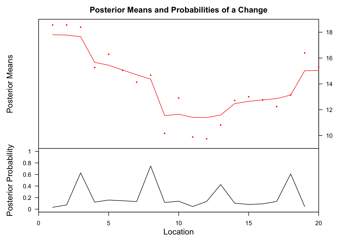
Highly non-linear (3 changes in regression)

set.seed(5)
x <- 1:50
z_nonoise <- c(0.1*x[1:10], 1.5-0.2*(x[11:25]-11), 
  -1.5 + 0.2*(x[26:45]-26), rep(1,5))
z <- z_nonoise + rnorm(50,0,0.2)
df <- data.frame(x = x, z = z)

plot(df$x, df$z, type = 'l', xlab = '', ylab = '')
lines(x = 1:10,y = 0.1*x[1:10], lwd = 3, col = 'red')
lines(x = 11:25, y = 1.5-0.2*(x[11:25]-11), lwd = 3, col = 'red')
lines(x = 26:45, y = -1.5 + 0.2*(x[26:45]-26), lwd = 3, col = 'red')
lines(x = 46:50, y = rep(1,5), lwd = 3, col = 'red')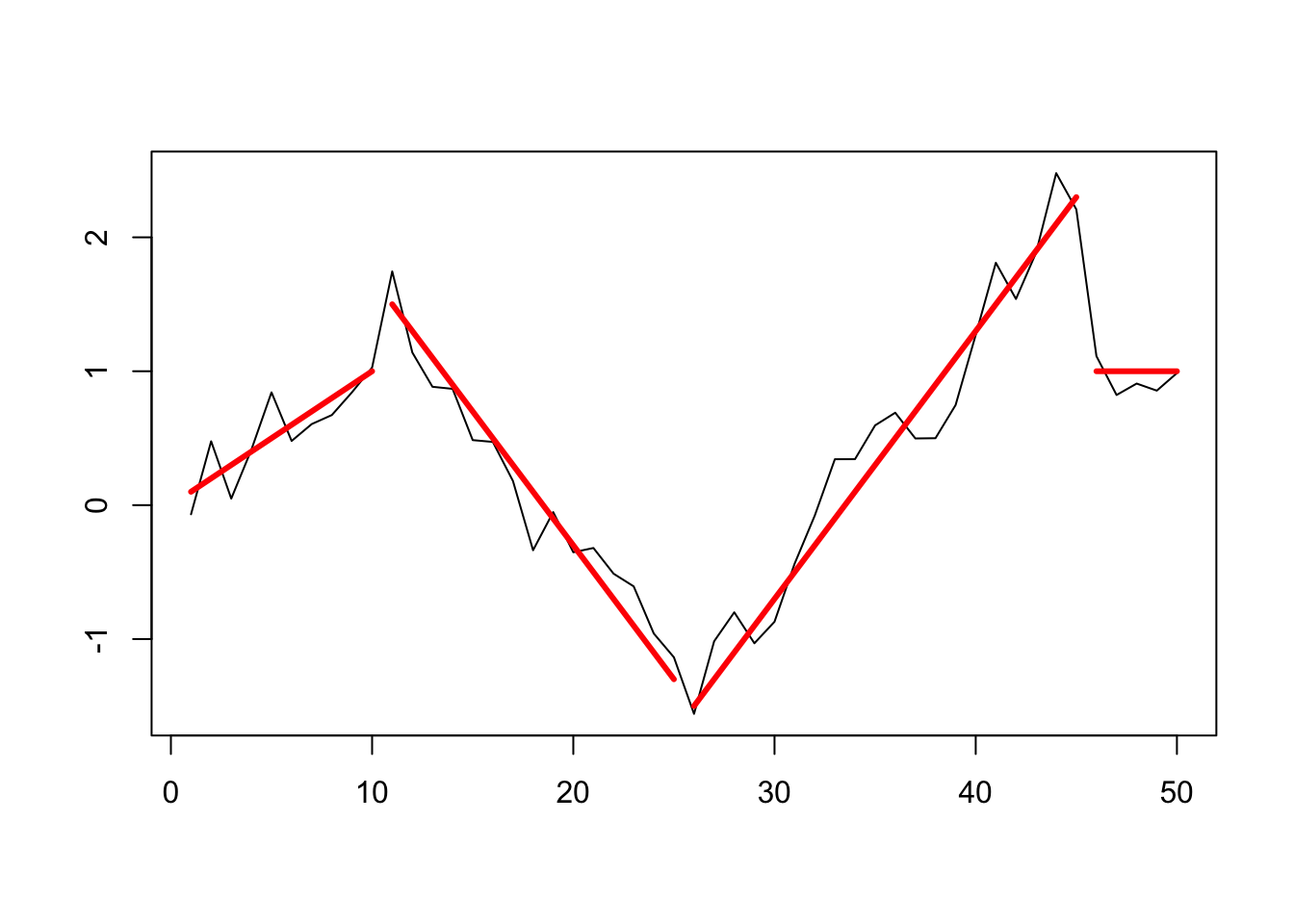

z_ts <- as.ts(df$z)

(changepoints at 10/11, 25/26, 45/46)

changepoint

Testing for 1 change point in mean

## Created Using changepoint version 2.2.2 
## Changepoint type      : Change in mean 
## Method of analysis    : AMOC 
## Test Statistic  : Normal 
## Type of penalty       : MBIC with value, 11.73607 
## Minimum Segment Length : 1 
## Maximum no. of cpts   : 1 
## Changepoint Locations :

Nothing found with the AMOC method.

Testing for several using PELT method and AIC penalty:

## Class 'cpt' : Changepoint Object
##        ~~   : S4 class containing 12 slots with names
##               cpttype date version data.set method test.stat pen.type pen.value minseglen cpts ncpts.max param.est 
## 
## Created on  : Fri Apr 26 15:58:35 2019 
## 
## summary(.)  :
## ----------
## Created Using changepoint version 2.2.2 
## Changepoint type      : Change in mean 
## Method of analysis    : PELT 
## Test Statistic  : Normal 
## Type of penalty       : AIC with value, 4 
## Minimum Segment Length : 1 
## Maximum no. of cpts   : Inf 
## Changepoint Locations : 17 32

Testing for several using PELT method and CROPS penalty:

## [1] "Maximum number of runs of algorithm = 8"
## [1] "Completed runs = 2"
## [1] "Completed runs = 3"
## [1] "Completed runs = 5"
## [1] "Completed runs = 7"

## Created Using changepoint version 2.2.2 
## Changepoint type      : Change in mean 
## Method of analysis    : PELT 
## Test Statistic  : Normal 
## Type of penalty       : CROPS with value, 1 25 
## Minimum Segment Length : 1 
## Maximum no. of cpts   : Inf 
## Changepoint Locations :  
## Number of segmentations recorded: 7  with between  0  and  6 changepoints.
##  Penalty value ranges from: 1  to  14.97552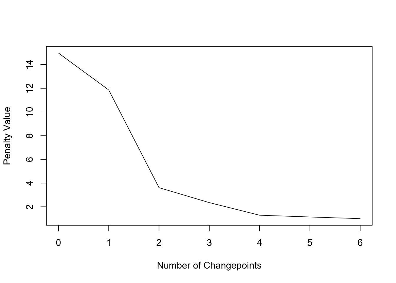

##      [,1] [,2] [,3] [,4] [,5] [,6]
## [1,]    4   16   23   31   39   45
## [2,]   17   23   31   39   45   NA
## [3,]   17   31   39   45   NA   NA
## [4,]   17   31   39   NA   NA   NA
## [5,]   17   32   NA   NA   NA   NA
## [6,]   39   NA   NA   NA   NA   NA
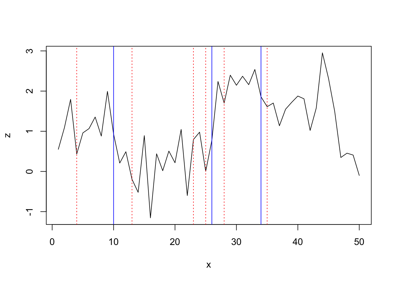
## [7,]   NA   NA   NA   NA   NA   NA

Changepoints at 17, 31, 39, and 45 detected:

plot(cpt2, ncpts = 4)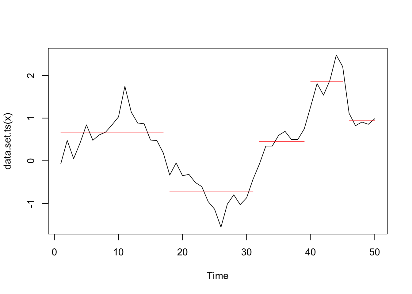

bcp

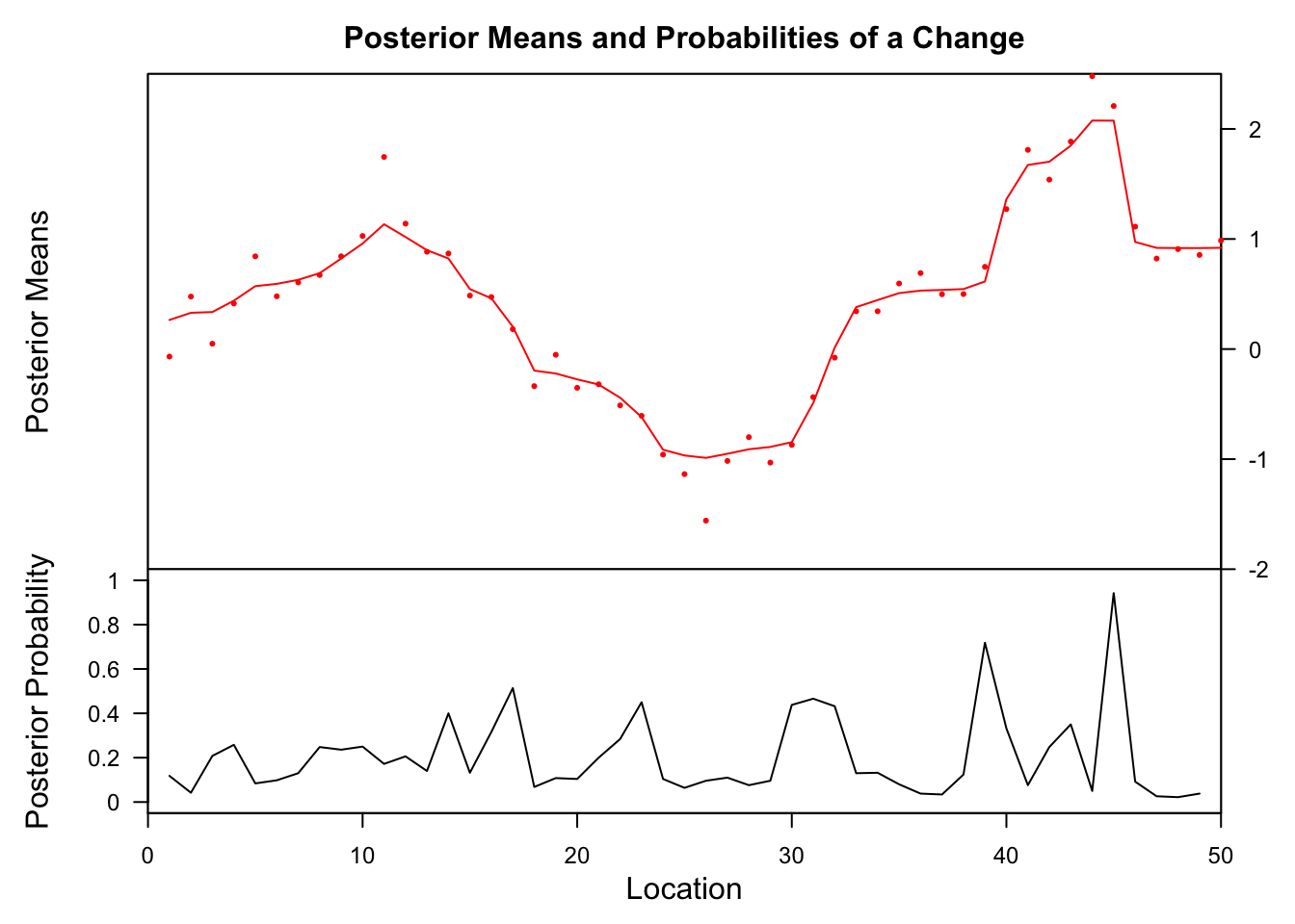
##    Probability        X1 id
## 39       0.718 0.6137687 39
## 45       0.942 2.0753858 45

The bcp method finds also at x = 39 and 45 change points but not before.

strucchange

Generalized fluctuation test

## 
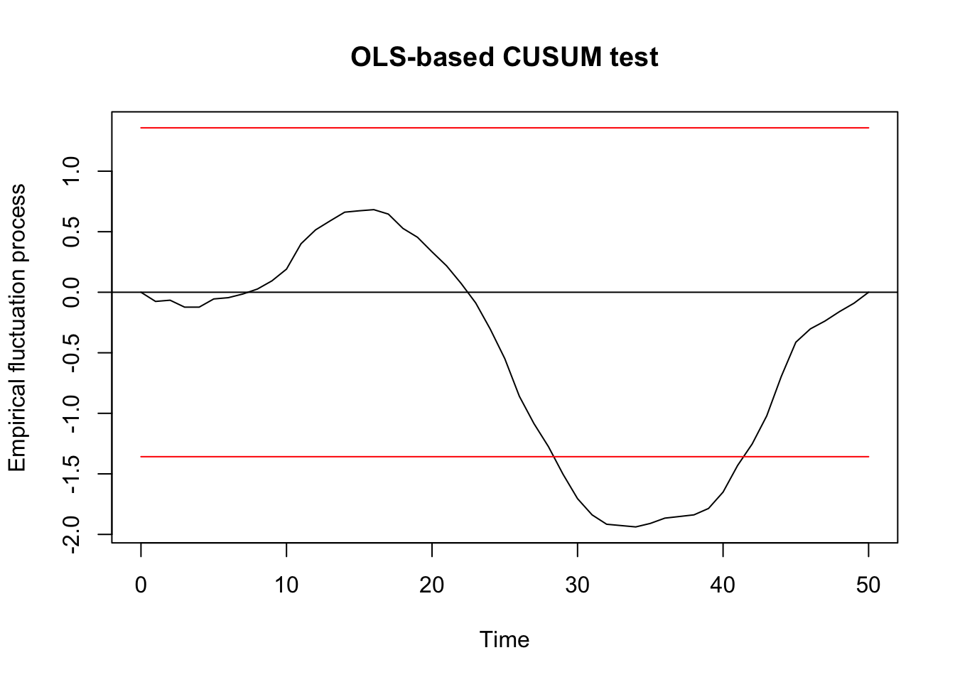
##  OLS-based CUSUM test
## 
## data:  ocus_mod
## S0 = 1.9381, p-value = 0.001093

F test

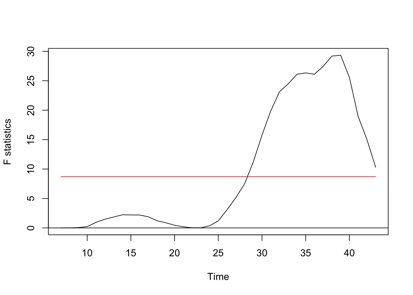
Regression breakpoints

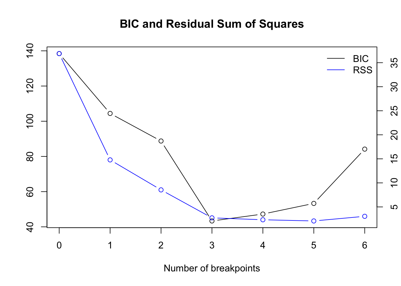
Get the optimal number numerically:

bpts_sum <- summary(bpts)
opt_brks <- opt_bpts(bpts_sum$RSS["BIC",])
opt_brks

## [1] 3

Location of breakpoint:

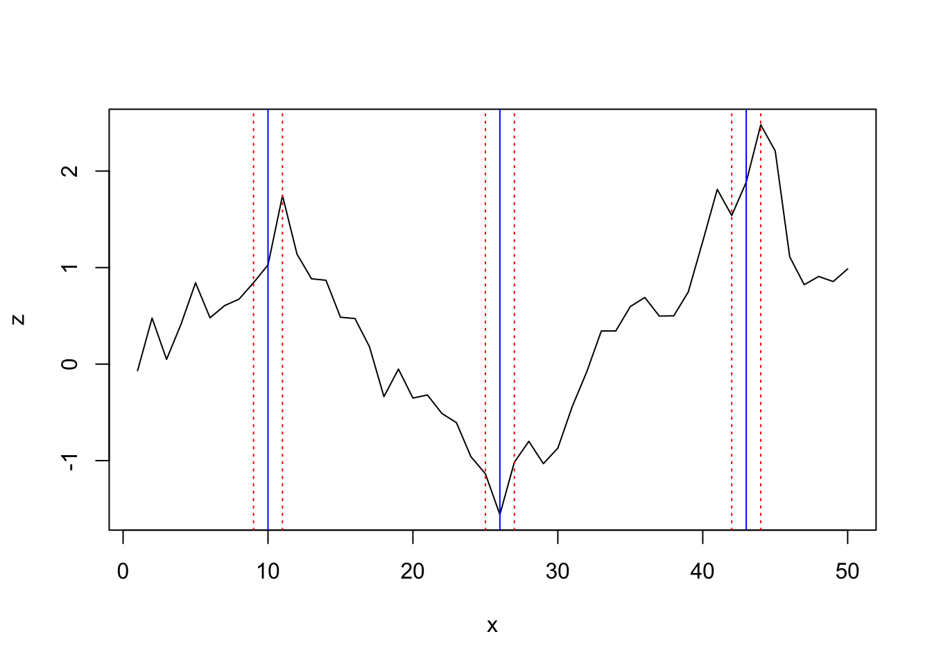
## [1] 10 26 43

The first 2 approaches in strucchange find one significant change point while the breakpoints algorithm finds 3:

segmented

Since I need to specify the number of change points directly in the function and i see already in the z~x plot several changes I provide 3 starting values (but for the purpose of performance evaluation will choose rather different ones):

lin_mod <- lm(z ~ x, data = df)
segm_mod <- segmented(lin_mod, seg.Z = ~x,
  psi=list(x=c(5,20,35)))
summary(segm_mod)$psi

##        Initial     Est.    St.Err
## psi1.x       5 11.02788 0.6905547
## psi2.x      20 26.00047 0.5059189
## psi3.x      35 43.99998 0.6284971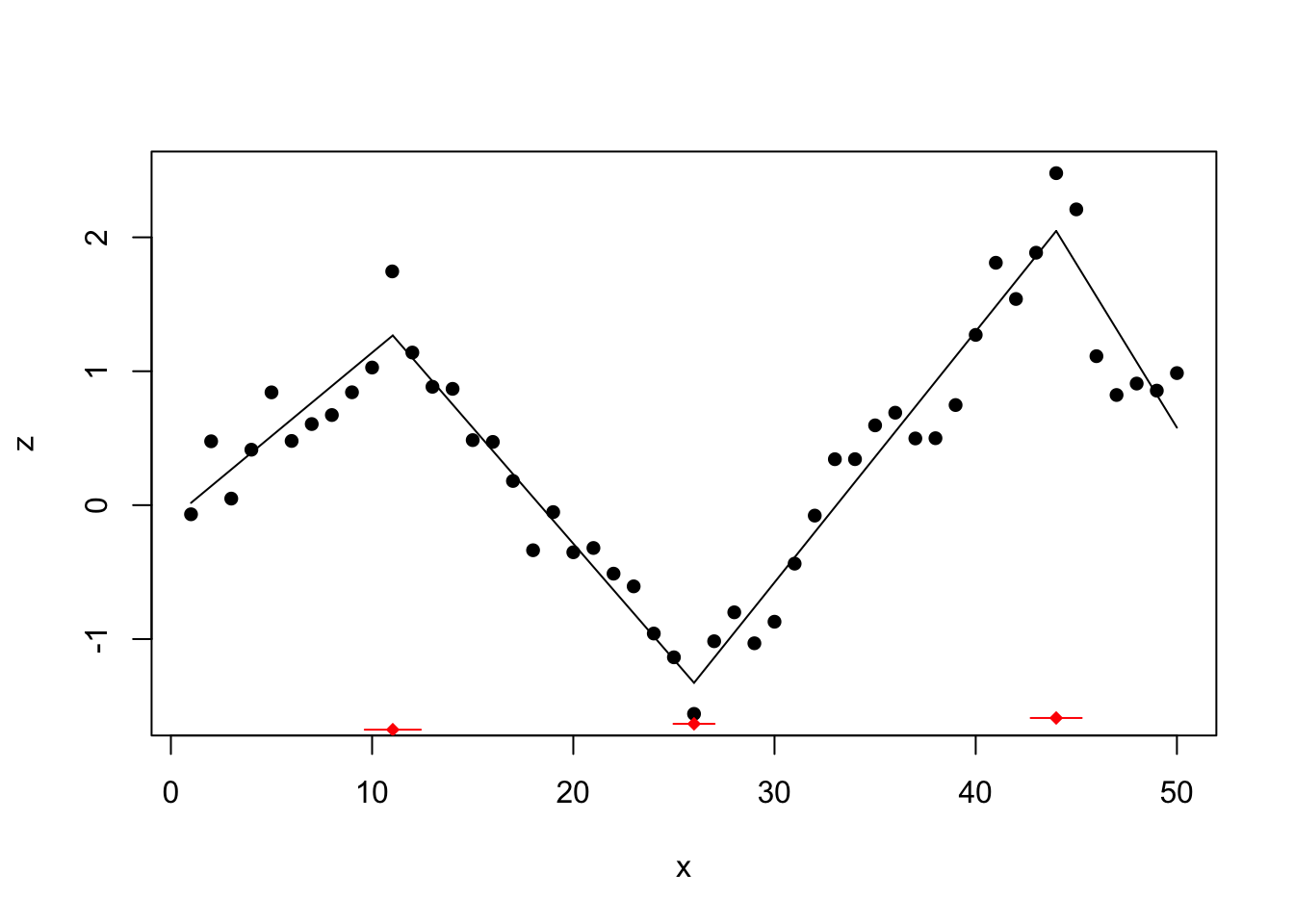

The segmented method finds the 3 change points at location 11, 26, and 44.

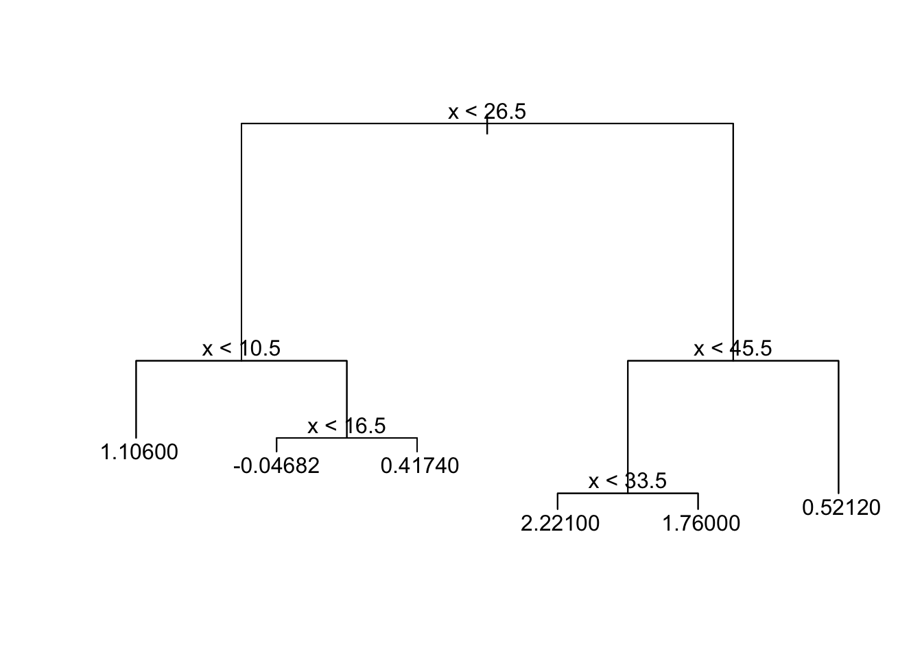
tree

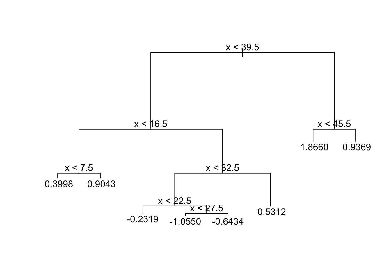
The tree methods finds 4 change points.

To cite this work: Otto, S.A. (2019, Sept.,28). Comparison of change point detection methods [Blog post]. Retrieved from https://www.marinedatascience.co/blog/2019/09/28/comparison-of-change-point-detection-methods/

Kortsch, S., Primicerio, R., Beuchel, F., Renaud, P.E., Rodrigues, J., Lønne, O.J. et al. (2012), Climate-driven regime shifts in Arctic marine benthos. Proc Nat Acad Sci U.S.A. 109:14052-14057, doi: 10.1073/pnas.1207509109 ↩
Samhouri, J.F., Andrews, K.S., Fay, G., Harvey, C.J., Hazen, E.L., Hennessey, S.M. et al. (2017), Defining ecosystem thresholds for human activities and environmental pressures in the California Current. Ecosphere 8:e01860, doi: 10.1002/ecs2.1860 ↩
Killick, R. & Eckley, I. A. (2014), changepoint: An R Package for Changepoint Analysis. J Stat Softw 58(3), 15p., doi: 10.18637/jss.v058.i03 ↩
Erdman, C. & Emerson, J. W. (2008), A fast Bayesian change point analysis for the segmentation of microarray data. Bioinformatics 24: 2143-2148, doi: 10.1093/bioinformatics/btn404 ↩
Zeileis, A., Leisch, F., Hornik, K. & Kleiber, C. (2002), strucchange: An R Package for Testing for Structural Change in Linear Regression Models. J Stat Softw 7(2), 38p., doi: 10.18637/jss.v007.i02 ↩
Muggeo, V.M.R. (2008), Segmented: an R package to fit regression models with broken-line relationships. R News 8/1, 20–25.↩
Cobb, G. W. (1978), The problem of the Nile: conditional solution to a change-point problem. Biometrika 65:243–51. doi: 10.1093/biomet/65.2.243 ↩

Comparison of change point detection methods

Overview

R packages for detecting change points

Summary

Take home message

Pros and cons of each method

Changes in mean

Changes in functional curves of relationships between X and Y

Detailed results and R code of detection performance under different scenarios

1 change in mean

Real data: Nile dataset

changepoint

bcp

strucchange

segmented

tree

Artificial data

changepoint

bcp

strucchange

segmented

tree

3 changes in mean

changepoint

bcp

strucchange

segmented

tree

Linear relationship (z~x) with 1 break

changepoint

bcp

strucchange

segmented

tree

Cubic decay function (z~x)

changepoint

bcp

strucchange

segmented

tree

Highly non-linear (3 changes in regression)

changepoint

bcp

strucchange

segmented

tree

Search

Categories

Tags