By Saskia | January 16, 2019
In this post I will present the oce package, which can be handy for marine data scientist working with oceanographical data. oce provides lots of functions to
- read oceanographic data,
- process the data specific to the measuring instrument, and
- visualize results following oceanographic conventions (using the base graphics).
The key function for importing data into R is ?read.oce(), which automatically recognizes the file type. If the recognition does not work, try the individual functions (e.g. read.ctd() for CTD files, read.odf() for ODF (Ocean Data Files) files, read.netcdf() for NetCDF files).
I won’t go into much detail on all the functions provided (for this see the reference manual or ?oce and then click on index at the bottom of the page). Instead, I will demonstrate you some plots you can create for specific datasets or purposes. The great advantage of this package is that you don’t need to wrangle your data into the typical data frame format for visualization and that it can handle many formats generated by typical oceanographical instruments!
The package also comes with few datasets included, e.g.
ctdwindsection(a hydrographic section)adp(ADP (acoustic-doppler profiler) dataset)echosounder(a degraded subsample of measurements that were made with a Biosonics scientific echosounder, as part of the St Lawrence Internal Wave Experiment (SLEIWEX) )landsat(a sample from the landsat satellite dataset)argo(holds data from the argo float ARGO 6900388 in the North Atlantic; FYI: argo floats are robots that float at different depths in the sea collecting information)lobo(sample lobo dataset obtained in the Northwest Arm of Halifax by Satlantic; a lobo is a complete turn-key water quality monitoring system that addresses the need for routine, robust, and accurate measurements)lisst(data from a LISST instruments, which is an in-situ optical laser diffraction instrument to measure particle size and concentration of suspended sediments)
Most other dataset have now been outsourced into the data package ocedata.
Plot CTD data
Lets look first at the CTD data included (CTD stands for Conductivity, Temperature, and Depth) :
library(oce)
data(ctd)
ctd
## ctd object, from file '/Users/kelley/git/oce/create_data/ctd/ctd.cnv', has data as follows.
## scan: 130, 131, ..., 309, 310 (length 181)
## time: 129, 130, ..., 308, 309 (length 181)
## pressure: 1.480, 1.671, ..., 43.903, 44.141 (length 181)
## depth: 1.468, 1.657, ..., 43.542, 43.778 (length 181)
## temperature: 14.225, 14.230, ..., 2.9190, 2.9194 (length 181)
## salinity: 29.921, 29.921, ..., 31.395, 31.393 (length 181)
## flag: 0, 0, ..., 0, 0 (length 181)summary(ctd)## CTD Summary
## -----------
##
## * Instrument: SBE 25
## * Temp. serial no.: 1140
## * Cond. serial no.: 832
## * File: "/Users/kelley/git/oce/create_data/ctd/ctd.cnv"
## * Original file: c:\seasoft3\basin\bed0302.hex
## * Start time: 2003-10-15 11:38:38
## * Sample interval: 1 s
## * Cruise: Halifax Harbour
## * Vessel: Divcom3
## * Station: Stn 2
## * Location: 44.684N 63.644W
## * Data
##
## Min. Mean Max. Dim. OriginalName
## scan 130 220 310 181 scan
## pressure [dbar] 1.48 22.885 44.141 181 pr
## depth [m] 1.468 22.698 43.778 181 depS
## temperature [°C, IPTS-68] 2.919 7.5063 14.237 181 t068
## salinity [PSS-78] 29.916 31.219 31.498 181 sal00
## flag 0 0 0 181 flag
##
## * Processing Log
## - 2017-09-09 17:00:27 UTC: `create 'ctd' object`
## - 2017-09-09 17:00:27 UTC: `read.ctd.sbe(file = file, processingLog = processingLog)`
## - 2017-09-09 17:00:27 UTC: `oce.edit(x = ctd, item = "startTime", value = ctd[["systemUploadTime"]], reason = "startTime in file has Y2K error", person = "Dan Kelley")`This dataset is a CTD profile measured at Halifax Harbour in 2003. The R object is obviously not in a data frame format but if you use an plotting function you don’t need to convert it as you will see next.
When loading the oce package, you can use the generic plot()function, which automatically recognizes the data type and applies the respective plotting method.
plot(ctd)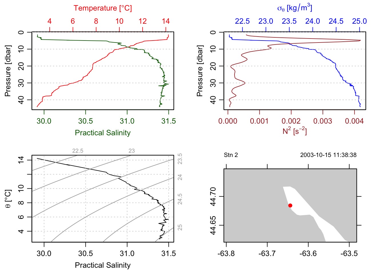
Figure 1: Four panels produced for CTD data.
The plot method for CTD data automatically generates several panels. If you want to plot only a subset, use the which argument:
plot(ctd, which = 1)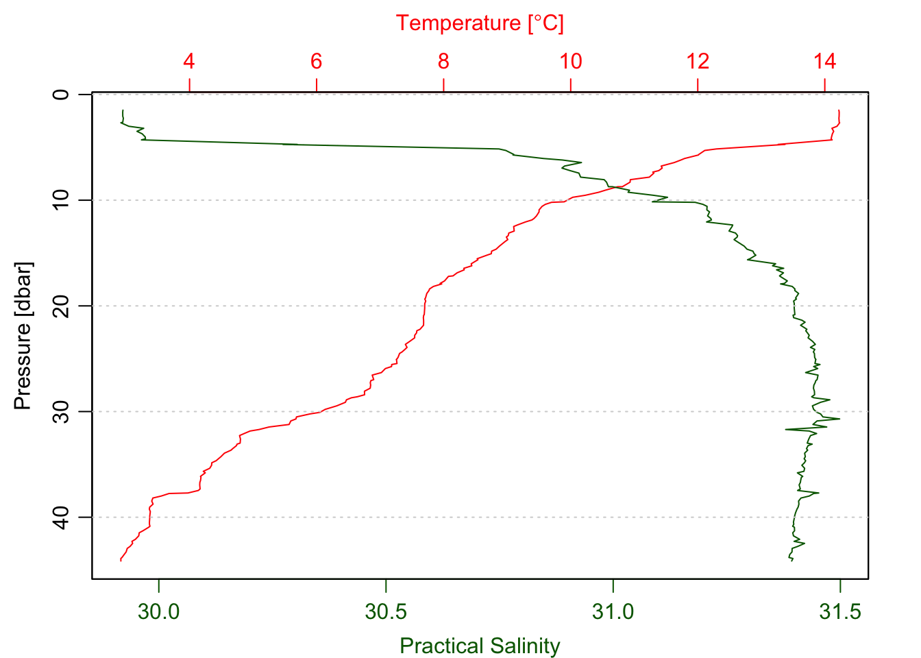
Figure 2: Only the temperature and salinity profile.
In the which argument you can provide a scalar or vector of desired plots. In fact, all plots that the package can produce have a number from 1 to 33, but not all can be generated with the same type of data. If the input data type is CTD, plot number 1,2,3, and 5 are produced (see also ?plot,ctd-method):
# same as plot(ctd):
plot(ctd, which = c(1,2,3,5))
The following would not make much sense or give an error:
plot(ctd, which=4)
plot(ctd, which=33)
Plot echosounder objects
If you have data from an an echosounder in this format
data(echosounder)
echosounder
## echosounder object, from file '/data/archive/sleiwex/2008/fielddata/2008-07-01/Merlu/Biosonics/20080701_163942.dt4', has data as follows.
## timeSlow: 2008-07-01 16:39:41, 2008-07-01 16:39:42, ..., 2008-07-01 16:42:49, 2008-07-01 16:42:50 (length 190)
## latitudeSlow: 47.879, 47.879, ..., 47.882, 47.882 (length 190)
## longitudeSlow: -69.724, -69.724, ..., -69.729, -69.729 (length 190)
## depth: 39.648, 38.933, ..., 2.4417, 1.7262 (length 54)
## time: 2008-07-01 16:39:41, 2008-07-01 16:39:41, ..., 2008-07-01 16:42:50, 2008-07-01 16:42:50 (length 389)
## latitude: 47.879, 47.879, ..., 47.882, 47.882 (length 389)
## longitude: -69.724, -69.724, ..., -69.729, -69.729 (length 389)
## a, a 389x54 array with value 131.375 at [1,1] positionsummary(echosounder)## Echosounder Summary
## -------------------
##
## * File source: "/data/archive/sleiwex/2008/fielddata/2008-07-01/Merlu/Biosonics/20080701_163942.dt4"
## * Transducer serial #: TX03022C
## * File type: DT4 pre v2.3
## * Beam type: single-beam
## * Channel: 1
## * Measurements: 2008-07-01 16:39:41 UTC to 2008-07-01 16:42:50 UTC
## * Sound speed: 1490.65 m/s
## * Pulse duration: 0.0004 s
## * Frequency: 418000.000000
## * Blanked samples: 57
## * Pings in file: 780
## * Samples per ping: 3399
## * Time ranges from 2008-07-01 16:39:41 to 2008-07-01 16:42:50 with 190 samples and mean increment 0.9998413 s
## * Data
##
## Min. Mean Max. Dim. OriginalName
## timeSlow 2008-07-01 18:39:41 2008-07-01 18:41:15 2008-07-01 18:42:50 190 -
## latitudeSlow [°N] 47.879 47.881 47.882 190 -
## longitudeSlow [°E] -69.729 -69.726 -69.724 190 -
## depth [m] 1.7262 20.687 39.648 54 -
## latitude [°N] 47.879 47.881 47.882 389 -
## longitude [°E] -69.729 -69.726 -69.724 389 -
## a 11.325 2492.3 364234 389x54 -
##
## * Processing Log
## - 2016-01-10 16:34:14 UTC: `create 'echosounder' object`
## - 2016-01-10 16:34:15 UTC: `read.echosounder(file = file, processingLog = processingLog)`
## - 2016-01-10 16:34:15 UTC: `subset.adp(x, subset=depth < 40)`
## - 2016-01-10 16:34:16 UTC: `decimate(x = echosounder, by = c(2, 40))`the would generate this plot:
plot(echosounder, which = 2, drawTimeRange = TRUE, drawBottom = TRUE)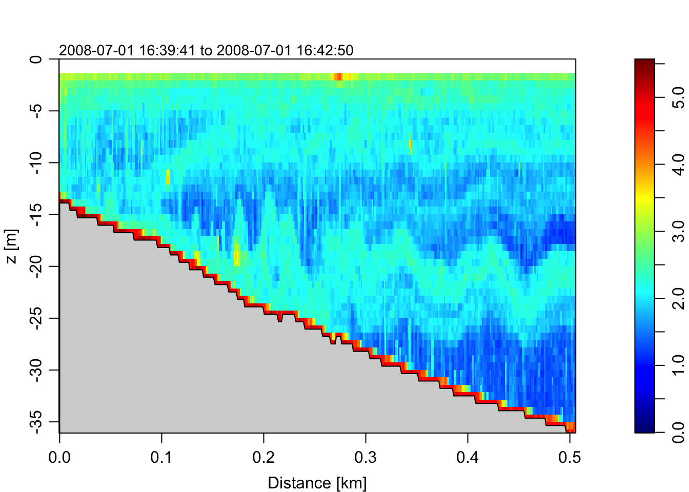
Figure 3: 3D contour plot of the echosounder.
Echo sounding is a type of sonar used to determine the depth of water by transmitting sound waves into water. But echo sounding can also refer to hydroacoustic “echo sounders” defined as active sound in water (sonar) used to study e.g. fish (commonly applied in fisheries).
In this plot you clearly see the seafloor, which reflects the signal strongest (hence, the red color). The color scale for the amplitude is log10-transformed and trimmed to zero.
Plot landsat objects
Landsat data can be downloaded from the USGS earthexplorer website. The following is a subset of the Landsat-8 image designated LC80080292014065LGN00, an image from March 2014 that covers Nova Scotia and portions of the Bay of Fundy and the Scotian Shelf:
data(landsat)
landsat
## Landsat object, ID LC80080292014065LGN00
## Data (bands or calculated):
## "aerosol" has dimension c(79,80)
## "blue" has dimension c(79,80)
## "green" has dimension c(79,80)
## "red" has dimension c(79,80)
## "nir" has dimension c(79,80)
## "swir1" has dimension c(79,80)
## "swir2" has dimension c(79,80)
## "panchromatic" has dimension c(158,160)
## "cirrus" has dimension c(79,80)
## "tirs1" has dimension c(79,80)
## "tirs2" has dimension c(79,80)plot(landsat, band = "temperature")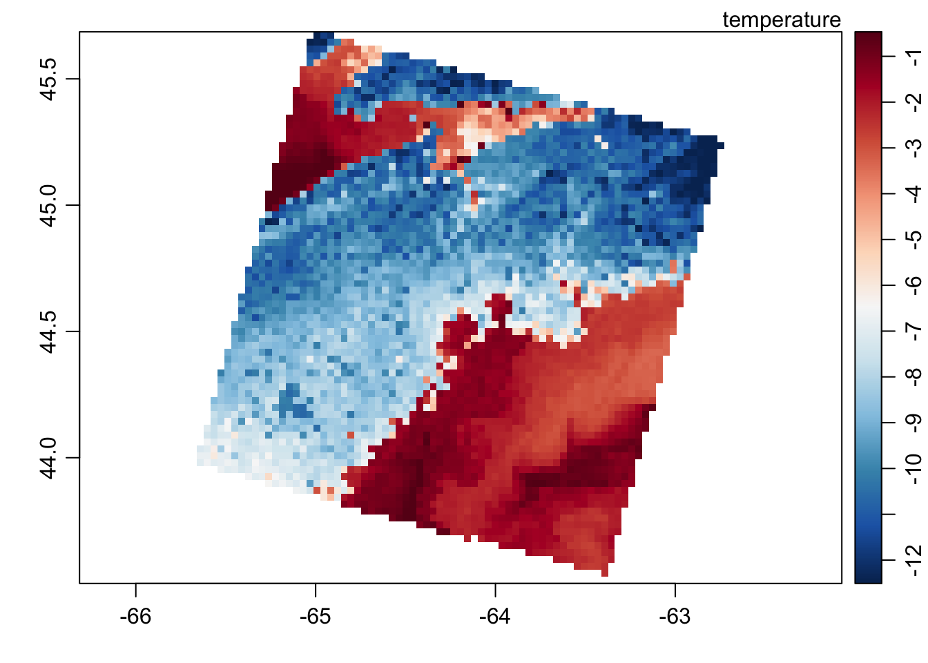
Figure 4: Image plot of the landsat data showing the temperature band.
Using band = "temperature" will plot an estimate of at-satellite brightness temperature, computed from the tirs1 band. Other band options for the Landsat-8 are "aerosol", "blue", "green", "red", "nir", "swir1", "swir2", "panchromatic", "cirrus", "tirs1", or "tirs2".
Plot coastline objects
oce provides a coastline dataset downloaded from Natural Earth. This dataset has a coarse resolution with a scale of 1:110M and 10,696 points, making it more suitable for world-scale plots plotted at a small size. If you want coastline files with a finer resolution use the ocedata package.
data(coastlineWorld)
coastlineWorld
## coastline object, from file '/Users/kelley/git/oce/create_data/coastline/ne_110m_admin_0_countries/ne_110m_admin_0_countries.shp', has data as follows.
## longitude: NA, 61.211, ..., 30.323, 29.839 (length 10766)
## latitude: NA, 35.65, ..., -22.272, -22.102 (length 10766)plot(coastlineWorld)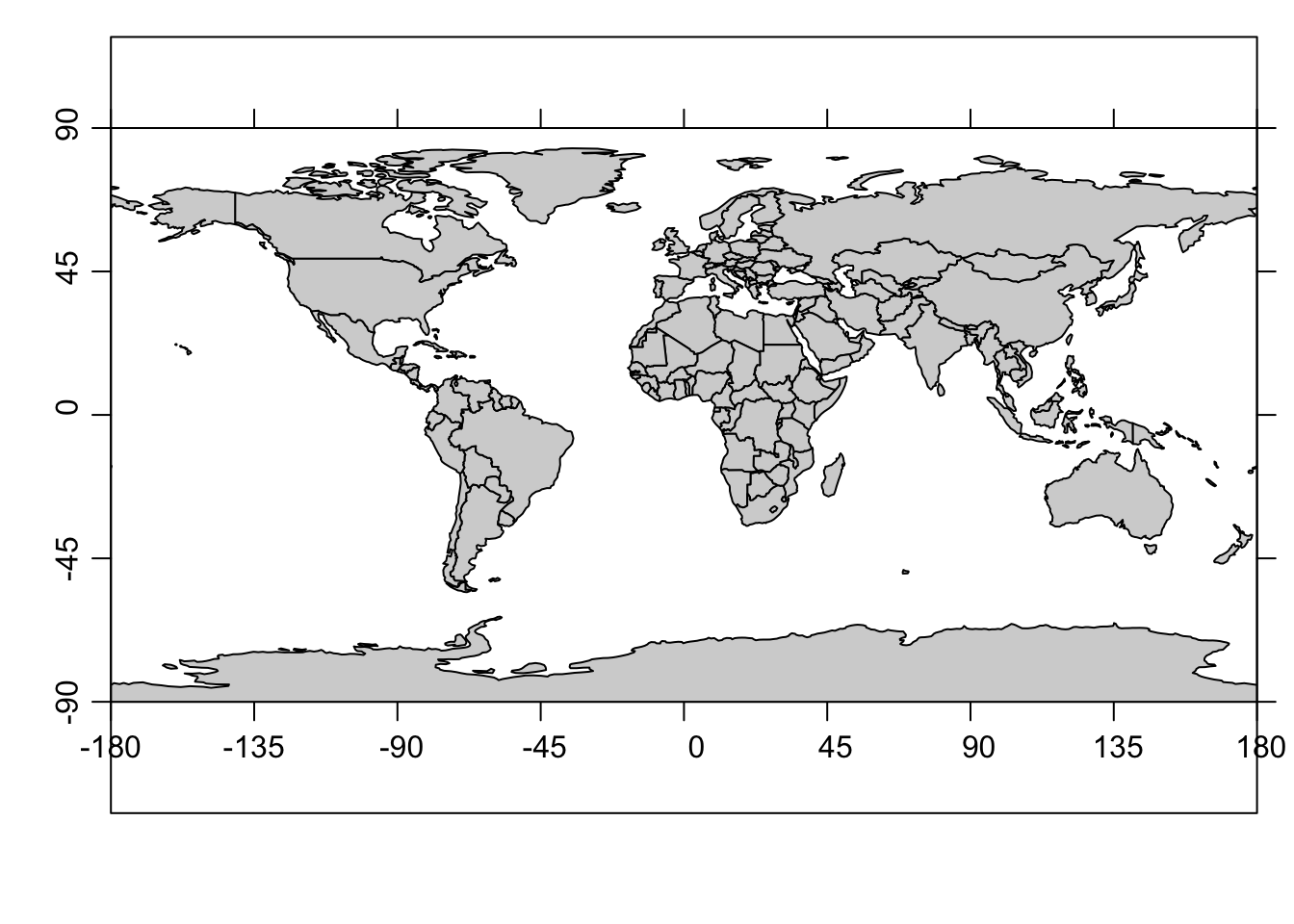
Figure 5: Generic coastline plot with a Cartesian projection.
If you want to create a map using a specific projection provided by the rgdal package, which makes it easy to add more items such as points, lines, contours or text, use the function mapPlot()from oce. Here I will plot the trajectory of the Cook’s Endeavour cruise (provided in the ocedata package) by adding the mapPoints() function:
# load the trajectory data
data(endeavour, package = "ocedata")

par(mar = rep(0.5, 4)) # that removes the margin
mapPlot(coastlineWorld, type = 'l', col = 'gray', projection = "+proj=moll")
# to add points use mapPoint()
mapPoints(endeavour$longitude, endeavour$latitude, pch = 20, col = 'red')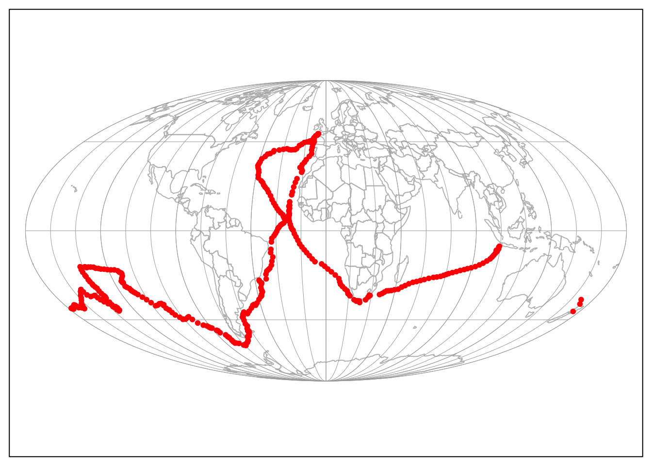
Figure 6: Global map with the Mollweide projection (default).
You can also add some colors for the topography. The required data is in the dataset topoWorld:
data(topoWorld)
topo <- decimate(topoWorld, 2) # coarsen grid: 4X faster plot
lon <- topo[["longitude"]]
lat <- topo[["latitude"]]
z <- topo[["z"]]
cm <- colormap(name = "gmt_globe")
drawPalette(colormap = cm)
par(mar = rep(0.5, 4))
mapPlot(coastlineWorld, type = 'l', col = 'gray', projection = "+proj=moll", grid = FALSE)
mapImage(lon, lat, z, colormap = cm)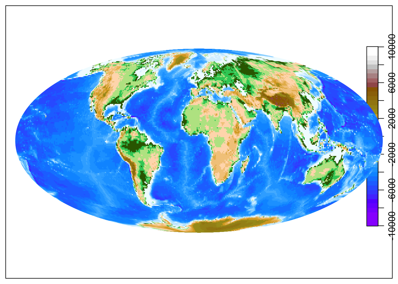
Figure 7: Global map with added topography.
When zooming into mid-latitude, the Lambert Conformal Conic projection is often used:
par(mar = c(2, 2, 1, 1))
lonlim <- c(-80, 0)
latlim <- c(20, 60)
mapPlot(coastlineWorld, projection = "+proj=lcc +lat_1=30 +lat_2=50 +lon_0=-40",
        col = "lightgray", longitudelim = lonlim, latitudelim = latlim)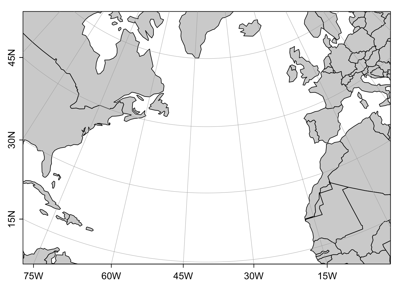
Figure 8: Map of the North-Atlantic based on the Lambert Conformal Conic projection.
See the ?mapPlot documentation on the different projections.
Global sea surface and temperature levels in 2013 from the World Ocean Atlas (WOA)
The ocedata package has a dataset named levitus, which stores sea-surface temperature (SST) and salinity (SSS) from the 2013 version of the World Ocean Atlas (WOA), commonly referred to as the “Levitus”" atlas (package version 0.1.3):
data(levitus, package = "ocedata")
par(mfrow = c(2,1))
imagep(levitus$longitude, levitus$latitude, levitus$SST, col = oceColorsJet, zlim = c(-2, 30))
imagep(levitus$longitude, levitus$latitude, levitus$SSS, col = oceColorsJet, zlim = c(20, 40))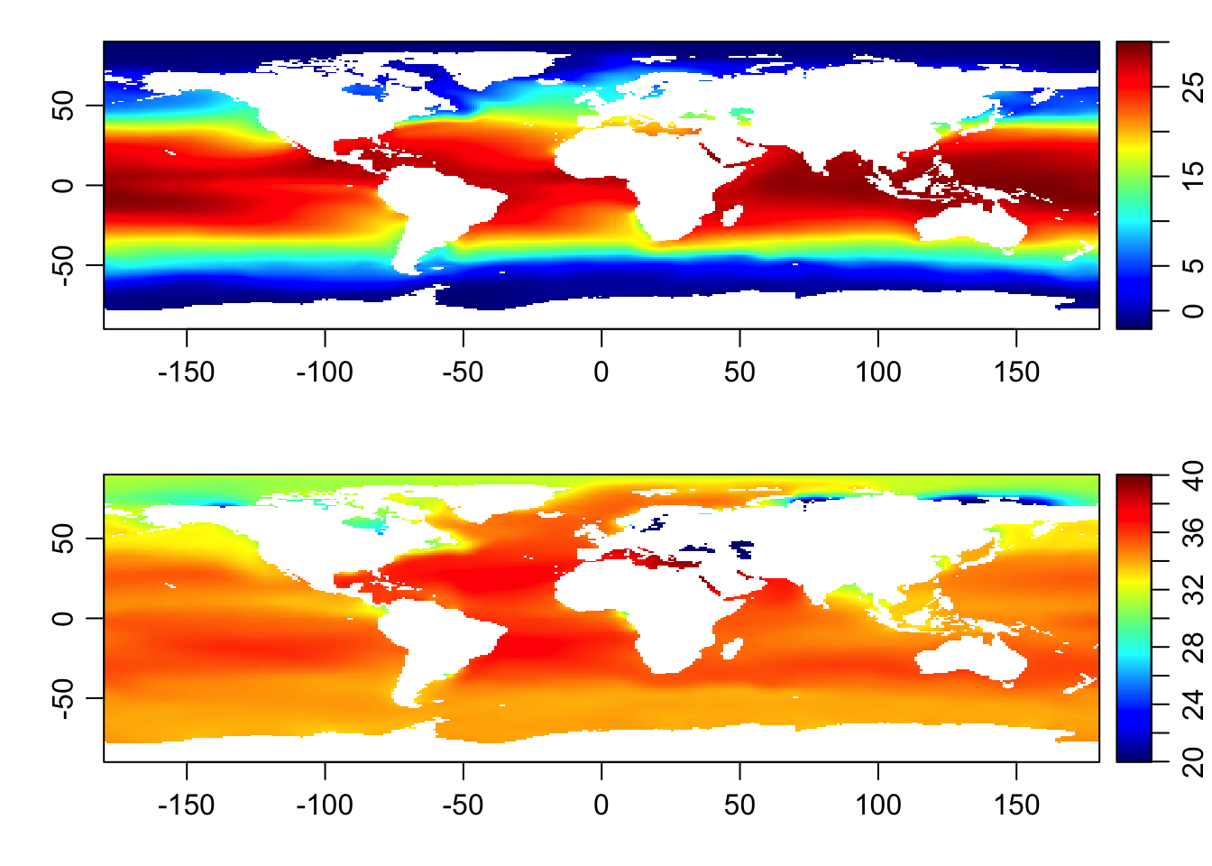
Figure 9: Distribution of annual temperature (top) and salinity (bottom) levels in 2013 (original source WOA).
More infos
For more information on the different plotting settings see the general plot help by typing one of the different plot methods, e.g. ?plot,ctd-method. Since the oce plot function produces various different type of plots, it is a bit tricky though to figure out which arguments are useful for which type of plot.
If you want to learn more about the package, I highly recommend the oce vignette and the github documentation page: https://cran.r-project.org/web/packages/oce/vignettes/oce.html. Dan Kelly, the author of the package, also wrote the book Oceanographic Analysis with R where the package is described in great detail.