By Saskia | January 7, 2019
This post has been stimulated by a discussion with a colleague who asked about the normalization method for the root mean square error (NRMSE) in the INDperform R package, which is based on the indicator testing framework outlined in my article (Otto et al. 2018)1. At the time of writing the article and package I simply used a common approach and didn’t test it much further. But sparked by this discussion I started to test it thoroughly (as you will see below), which will make me revise the package.
The Root Mean Square Error (RMSE)
In statistical modeling and particularly regression analyses, a common way of measuring the quality of the fit of the model is the RMSE (also called Root Mean Square Deviation), given by $$RMSE = \sqrt\frac{\sum_{i=1}^{n} \left(y_{i} - \hat{y}\right)^{2}} {n}$$
where \(y_{i}\) is the ith observation of y and ŷ the predicted y value given the model. If the predicted responses are very close to the true responses the RMSE will be small. If the predicted and true responses differ substantially - at least for some observations - the RMSE will be large. A value of zero would indicate a perfect fit to the data. Since the RMSE is measured on the same scale, with the same units as \(y\), one can expect 68% of the y values to be within 1 RMSE - given the data is normally distributed.
So calculating the MSE helps comparing different models that are based on the same y observations. But what if
- one wants to compare model fits of different response variables?
- the response variable y is modified in some models, e.g. standardized or sqrt- or log-transformed?
- And does the slitting of data into a training and test dataset (after the modification) and the RMSE calculation based on the test data an effect on point 1. and 2.?
The first two points are typical issues when comparing ecological indicator performances and the latter, so-called validation set approach2, is pretty common in statistical and machine learning. One solution to overcome these barriers - as done in INDperform - is to calculate the Normalized RMSE.
Normalized Root Mean Square Error (NRMSE)
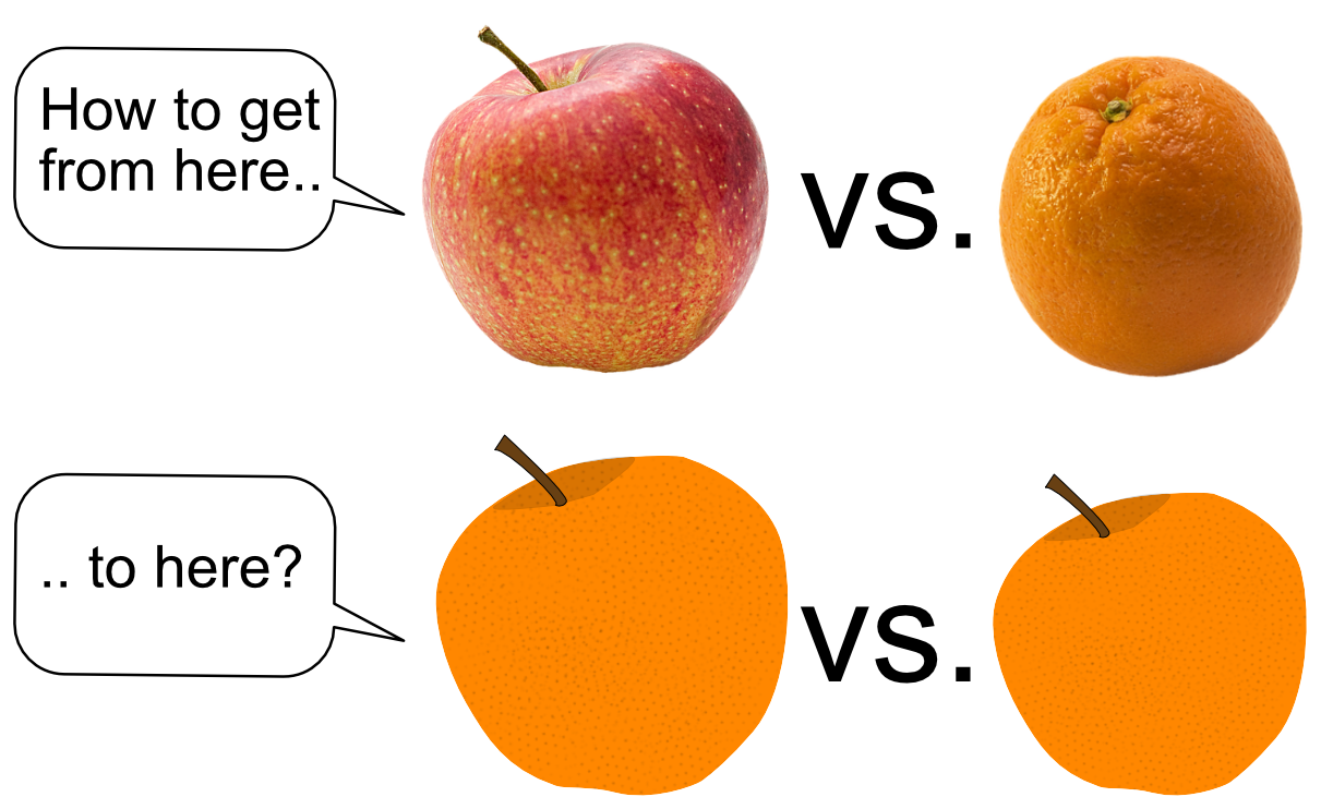
There is a saying that apples shouldn’t be compared with oranges or in other words, don’t compare two items or group of items that are practically incomparable. But the lack of comparability can be overcome if the two items or groups are somehow standardized or brought on the same scale. For instance, when comparing the variances of two groups that are overall very different, such as the variance in size of bluefin tuna and blue whales, the coefficient of variation (CV) is the method of choice: the CV simply represents the variance of each group standardized by its group mean:
tuna <- c(150, 200, 250, 210,180, 305)
whale <- c(2300, 2000, 2250, 1900, 2100)
c( var(tuna), var(whale) )
## [1] 3004.167 28000.000c( sd(tuna), sd(whale) )## [1] 54.81028 167.33201c( var(tuna)/mean(tuna), var(whale)/mean(whale) )## [1] 13.91892 13.27014While in absolute values the individual whales differ from each other much more than the tuna fish, this variation is rather small relative to the overall size of the whales and then comparable to tuna.
In the same way, normalizing the RMSE facilitates the comparison between datasets or models with different scales. You will find, however, various different methods of RMSE normalizations in the literature:
You can normalize by
the mean: \(NRMSE = \frac{RMSE}{\bar{y}}\) (similar to the CV and applied in INDperform)
the difference between maximum and minimum: \(NRMSE = \frac{RMSE}{y_{max} - y_{min}}\),
the standard deviation: \(NRMSE = \frac{RMSE}{\sigma}\), or
the interquartile range; \(NRMSE = \frac{RMSE}{Q1 - Q3}\), i.e. the difference between 25th and 75th percentile,
of observations.
If the response variables has few extreme values, choosing the interquartile range is a good option as it is less sensitive to outliers. But how do these methods compare in terms of data transformation and the validation set approach?
Comparison of different RMSE normalizations under different data treatments
In the following comparison I will compare the 4 methods using the original, standardized, sqrt- and log-transformed dataset. First I will use the full dataset to train and test the model (via RNMSE), then split the data into a training and test subset. In this case, I will assume the data is a time series and the validation is performed on the last years (so no random splitting) as done in many time series predictions.
To be able to link the results of the comparison to the approach in INDperform I will also use here Generalized Additive Models (GAM)3 based on the mgcv package.
Self-made functions
library(mgcv)
library(tidyverse)
Hand-made NRMSE function:
nrmse_func <-  function(obs, pred, type = "sd") {

    squared_sums <- sum((obs - pred)^2)
    mse <- squared_sums/length(obs)
    rmse <- sqrt(mse)
    if (type == "sd") nrmse <- rmse/sd(obs)
    if (type == "mean") nrmse <- rmse/mean(obs)
    if (type == "maxmin") nrmse <- rmse/ (max(obs) - min(obs))
    if (type == "iq") nrmse <- rmse/ (quantile(obs, 0.75) - quantile(obs, 0.25))
    if (!type %in% c("mean", "sd", "maxmin", "iq")) message("Wrong type!")
    nrmse <- round(nrmse, 3)
 return(nrmse)

}
The following comp_func() function does the actual modeling, prediction and NRMSE calculation for the different Y’s on the full or split data (split = TRUE, taking the last 5 observations for testing):
# helper function for comp_func()
lowest <- function(x) {
    x <- paste0(names(which(x == min(x))), collapse = ",")
    return(x)
}

comp_func <- function(y, x, split = TRUE, test_n = 5) {

  df <- data.frame(x = x,   y = y)

  # Add y transformations
  df$y_stand = as.vector(scale(df$y))
  df$y_sqrt = sqrt(df$y)
  df$y_log = log(df$y)

  # Split time series into training/test data (or not)
  if (split == TRUE) {
    df_train <- df[1:(nrow(df) - test_n), ]
    df_test <- df[(nrow(df_train)+1):nrow(df), ]
  } else {
    df_train <- df
    df_test <- df
  }

  # Models
  m1 <- gam(y ~ s(x, k = 4), data = df_train)
  m2 <- gam(y_stand ~ s(x, k = 4), data = df_train)
  m3 <- gam(y_sqrt ~ s(x, k = 4), data = df_train)
  m4 <- gam(y_log ~ s(x, k = 4), data = df_train)

  # Predictions
  df_comp <- df_test
  df_comp$pred <- as.vector(predict(m1, newdata = df_test))
  df_comp$pred_stand <- as.vector(predict(m2, newdata = df_test))
  df_comp$pred_sqrt <- as.vector(predict(m3, newdata = df_test))
  df_comp$pred_log <- as.vector(predict(m4, newdata = df_test))

  # Back-transform the predictions for y_sqrt and y_log for comparison
  df_comp$pred_sqrt_b<- df_comp$pred_sqrt ^2
  df_comp$pred_log_b <- exp(df_comp$pred_log)

  # Reorder variables for NRMSE loop (add y twice for back-transformed predictions)
  df_loop <- df_comp[ ,c(2,3,4,2,5,2,6:8,10,9,11)]

  # Calculate NRMSE for 4 different types of normalization
  type_vec <- c("mean", "sd", "maxmin", "iq")
  out <- data.frame(
    type = type_vec,
    y = rep(NA, 4), y_stand = rep(NA, 4),
    y_sqrt = rep(NA, 4), y_sqrt_b = rep(NA, 4),
    y_log = rep(NA, 4), y_log_b = rep(NA, 4)
  )
  for (i in 1:4) {
    for (k in 1:6) {
      out[i, k+1] <- nrmse_func(obs = df_loop[ ,k], pred = df_loop[ ,k+6], type = type_vec[i])
    }
  }
  # Add column indicating whether y, y_sqr, y_sqr_b, y_log or y_log_b2
  # has the lowest NRMSE
  out$lowest <- unlist(apply(out[ ,c(2,4:7)], 1, FUN = lowest))
  out

  return(out)
}
Simulated datasets
set.seed(1)
simdat <- data.frame(
    x1 = 1:20,
  # add polynomial of second order to produce a non-linear decline
    y1 = 170 + 2.5*1:20 - 0.5* (1:20)^2  + rnorm(20, 0, 40),
  x2 = sample(seq(15, 30, 0.01), 20)
)
# produce linear positive trend
simdat$y2 <- 50 + 1.5 * simdat$x2 + rnorm(20, 0, 8)
# produce same trend but with increasing variance
simdat$y3 <- simdat$y2
for (i in 1:20) {
  noise <- rnorm(1, 0, sd = 2*i)
  simdat$y3[i] <- simdat$y3[i] + noise
}

par(mfrow = c(1,3))
plot(simdat$y1 ~ simdat$x1)
plot(simdat$y2 ~ simdat$x2)
plot(simdat$y3 ~ simdat$x2)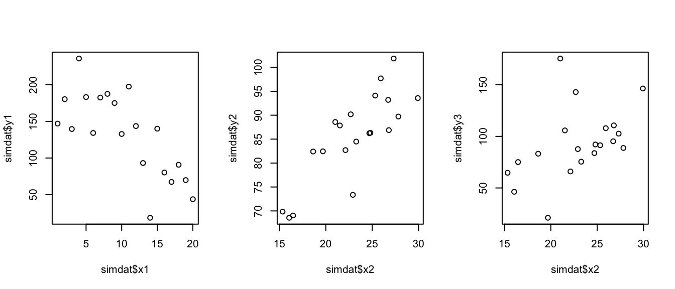
Comparison
Full data
fd1 <- comp_func(x = simdat$x1, y = simdat$y1, split = FALSE)
fd1 %>%
  knitr::kable(
    format = "html", align = "c",
    col.names = c("Type", "Raw Y", "Standardized", "Sqrt-transf.", "Sqrt-backtransf.",
    "Log-transf.", "Log-backtransf.", "Lowest NRMSE"),
    caption = "Non-linear (full) dataset"
  ) %>%
  kableExtra::kable_styling(
    bootstrap_options = c("striped", "condensed", "responsive")
)| Type | Raw Y | Standardized | Sqrt-transf. | Sqrt-backtransf. | Log-transf. | Log-backtransf. | Lowest NRMSE |
|---|---|---|---|---|---|---|---|
| mean | 0.256 | 2.90688e+15 | 0.159 | 0.264 | 0.094 | 0.310 | y_log |
| sd | 0.590 | 5.90000e-01 | 0.631 | 0.608 | 0.725 | 0.713 | y |
| maxmin | 0.156 | 1.56000e-01 | 0.160 | 0.161 | 0.174 | 0.188 | y |
| iq | 0.365 | 3.65000e-01 | 0.436 | 0.376 | 0.617 | 0.441 | y |
fd2 <- comp_func(x = simdat$x2, y = simdat$y2, split = FALSE) | Type | Raw Y | Standardized | Sqrt-transf. | Sqrt-backtransf. | Log-transf. | Log-backtransf. | Lowest NRMSE |
|---|---|---|---|---|---|---|---|
| mean | 0.060 | 7.994036e+14 | 0.030 | 0.060 | 0.014 | 0.060 | y_log |
| sd | 0.554 | 5.540000e-01 | 0.543 | 0.552 | 0.533 | 0.551 | y_log |
| maxmin | 0.155 | 1.550000e-01 | 0.154 | 0.155 | 0.152 | 0.154 | y_log |
| iq | 0.608 | 6.080000e-01 | 0.610 | 0.606 | 0.615 | 0.604 | y_log_b |
fd3 <- comp_func(x = simdat$x2, y = simdat$y3, split = FALSE) | Type | Raw Y | Standardized | Sqrt-transf. | Sqrt-backtransf. | Log-transf. | Log-backtransf. | Lowest NRMSE |
|---|---|---|---|---|---|---|---|
| mean | 0.321 | -5.439201e+15 | 0.168 | 0.323 | 0.085 | 0.328 | y_log |
| sd | 0.865 | 8.650000e-01 | 0.849 | 0.870 | 0.848 | 0.885 | y_log |
| maxmin | 0.194 | 1.940000e-01 | 0.184 | 0.195 | 0.179 | 0.198 | y_log |
| iq | 0.966 | 9.660000e-01 | 0.976 | 0.971 | 1.104 | 0.987 | y |
SUMMARY:
- NRMSE of the standardized Y is
- close to zero when using type mean → this is not surprising given the nature of the standardization itself (the “standardization”, also called “normalization” or “z-transformation”, standardizes the data to a mean of zero and a standard deviation of 1).
- exactly the same than the NRMSE for the original Y when using the other normalization methods
- NRMSE of the transformed Ys always deviates from the NRMSE of the original Y, no matter which method was used (except for the second dataset, when using the mean); however, back-transforming does bring the NRMSE closer to the original NRMSE! The degree of deviation depends also on the Y~X relationship and, hence, the model (smaller in the linear datasets)!
- Log-transforming Y deviates much greater and often leads to a lower NRMSE, although this also depends on the Y~X relationship.
- No clear pattern in the performance differences between the four normalization types (unless variables are standardized).
Test data
td1 <- comp_func(x = simdat$x1, y = simdat$y1, split = TRUE, test_n = 5) | Type | Raw Y | Standardized | Sqrt-transf. | Sqrt-backtransf. | Log-transf. | Log-backtransf. | Lowest NRMSE |
|---|---|---|---|---|---|---|---|
| mean | 0.268 | -0.306 | 0.150 | 0.288 | 0.089 | 0.340 | y_log |
| sd | 1.077 | 1.077 | 1.147 | 1.157 | 1.367 | 1.365 | y |
| maxmin | 0.402 | 0.402 | 0.431 | 0.431 | 0.518 | 0.509 | y |
| iq | 1.469 | 1.469 | 1.675 | 1.578 | 2.164 | 1.863 | y |
td2 <- comp_func(x = simdat$x2, y = simdat$y2, split = TRUE, test_n = 5) | Type | Raw Y | Standardized | Sqrt-transf. | Sqrt-backtransf. | Log-transf. | Log-backtransf. | Lowest NRMSE |
|---|---|---|---|---|---|---|---|
| mean | 0.058 | -2.271 | 0.030 | 0.060 | 0.014 | 0.063 | y_log |
| sd | 0.572 | 0.572 | 0.578 | 0.593 | 0.583 | 0.615 | y |
| maxmin | 0.230 | 0.230 | 0.233 | 0.238 | 0.236 | 0.247 | y |
| iq | 0.793 | 0.793 | 0.833 | 0.822 | 0.878 | 0.852 | y |
td3 <- comp_func(x = simdat$x2, y = simdat$y3, split = TRUE, test_n = 5) | Type | Raw Y | Standardized | Sqrt-transf. | Sqrt-backtransf. | Log-transf. | Log-backtransf. | Lowest NRMSE |
|---|---|---|---|---|---|---|---|
| mean | 0.550 | 6.792 | 0.306 | 0.554 | 0.161 | 0.559 | y_log |
| sd | 0.928 | 0.928 | 0.879 | 0.934 | 0.855 | 0.944 | y_log |
| maxmin | 0.361 | 0.361 | 0.340 | 0.363 | 0.335 | 0.367 | y_log |
| iq | 0.822 | 0.822 | 0.894 | 0.827 | 1.102 | 0.836 | y |
SUMMARY:
- Overall, deviations between different data treatments are much greater when training the model on a training subset and computing the NRMSE for a test subset.
- Similar to using the full data, NRMSEs of the original and standardized Y are the same, except when using the mean to normalize.
- But beside the standardization, performances of the four normalization are comparable, even when using only a test subset.
- Again, transformed Ys always differ in their NRMSE from the original Y and this difference is
- greater in the log-transformed Ys
- but: back-transforming does not always reduce the difference as shown in the second, linear dataset with constant variance.
Conclusion
So what did we learn from this simulation?
First and foremost, comparing model performances between different response variables is not that trivial and there is no normalization method (of the one tested here) that is obviously superior. But there are a few implications that data analysts should bear in mind when computing the NRMSE for performance comparison:
- NRMSE should be better computed on the untransformed scale. That means, if the response variable Y was transformed prior to the modeling, to e.g. linearize the relationship, reduce heterogeneity, etc., the predicted values should be back-transformed and compared with the observed raw data when computing the NRMSE.
- Using the mean to normalize the NRMSE is ok as long as you compare models that are based on the same response variable and data treatment.
- Otherwise, use any of the other 3 methods:
- While maxmin is said to be more sensitive to the sample size, I did not find a big difference to the other methods, even when using a sample size of 5 (when splitting the data).
- The interquartile range is said to be less sensitive to extreme values → since I didn’t have extreme values in the simulated data I didn’t find a strong difference to the other methods
But who actually cares about comparing model performances of different response variables? One good example (where the package was made for) is the development of ecological indicators. One major criterion is the robustness or predictability given certain environmental changes. This could be quantified from a statistical model, in which the indicator is modelled as a function of specific environmental variable or pressure, by using the RMSE on the test data. To compare the robustness of different indicators, that are often on different scales and differently treated prior to the modeling, normalizing the NRMSE would be needed.
If the NRMSE is further categorized into let’s say low, medium or high performance, using the standard deviation to normalize could be a good option for the following reason: The sd-based NRMSE represent the ratio between the variation not explained by the regression vs the overall variation in Y. If the regression explains all of the variation in Y, nothing gets unexplained and the RMSE, and consequently NRMSE is zero. If the regression explains some part and leaves some other unexplained, which is at a similar scale than the overall variation, the ratio will be around 1. Anything beyond will indicate a much greater variation or noise than in the variable itself and consequently a low predictability.
Stay tuned for the next update of INDperform, where I will revise the NRMSE calculation (most likely using the sd method) and the cut-offs for scoring!
To cite this work: Otto, S.A. (2019, Jan.,7). How to normalize the RMSE [Blog post]. Retrieved from https://www.marinedatascience.co/blog/2019/01/07/normalizing-the-rmse/
Otto, S.A., Kadin, M., Casini, M., Torres, M.A. & Blenckner, T. (2018). A quantitative framework for selecting and validating food web indicators. Ecological Indicators, 84, 619-631, doi: 10.1016/j.ecolind.2017.05.045↩
James, G., Witten, D., Hastie, T. & Tibshirani, R. (2013). An Introduction to Statistical Learning - with Applications in R. Springer, New York.↩
Hastie, T.J. & Tibshirani, R.J. (1990). Generalized Additive Models. Chapman & Hall / CRC, Boca Raton, 352 p.↩